
By:
Arip Nurahman
Department of Physics
Faculty of Sciences and Mathematics, Indonesia University of Education
and
Follower Open Course Ware at Massachusetts Institute of Technology
Cambridge, USA
Department of Physics
http://web.mit.edu/physics/
http://ocw.mit.edu/OcwWeb/Physics/index.htm
&
Aeronautics and Astronautics Engineering
http://web.mit.edu/aeroastro/www/
http://ocw.mit.edu/OcwWeb/Aeronautics-and-Astronautics/index.htm


| Fourier transforms |
|---|
| Continuous Fourier transform |
| Fourier series |
| Discrete Fourier transform |
| Discrete-time Fourier transform |
In mathematics, Fourier analysis is a subject area which grew out of the study of Fourier series. The subject began with trying to understand when it was possible to represent general functions by sums of simpler trigonometric functions. The attempt to understand functions (or other objects) by breaking them into basic pieces that are easier to understand is one of the central themes in Fourier analysis. Fourier analysis is named after Joseph Fourier who showed that representing a function by a trigonometric series greatly simplified the study of heat propagation.
Today the subject of Fourier analysis encompasses a vast spectrum of mathematics with parts that, at first glance, may appear quite different. In the sciences and engineering the process of decomposing a function into simpler pieces is often called an analysis. The corresponding operation of rebuilding the function from these pieces is known as synthesis. In this context the term Fourier synthesis describes the act of rebuilding and the term Fourier analysis describes the process of breaking the function into a sum of simpler pieces. In mathematics, the term Fourier analysis often refers to the study of both operations.
In Fourier analysis, the term Fourier transform often refers to the process that decomposes a given function into the basic pieces. This process results in another function that describes how much of each basic piece are in the original function. It is common practice to also use the term Fourier transform to refer to this function. However, the transform is often given a more specific name depending upon the domain and other properties of the function being transformed, as elaborated below. Moreover, the original concept of Fourier analysis has been extended over time to apply to more and more abstract and general situations, and the general field is often known as harmonic analysis.
Each transform used for analysis (see list of Fourier-related transforms) has a corresponding inverse transform that can be used for synthesis.
Contents
|
Applications
This wide applicability stems from many useful properties of the transforms:
- The transforms are linear operators and, with proper normalization, are unitary as well (a property known as Parseval's theorem or, more generally, as the Plancherel theorem, and most generally via Pontryagin duality)(Rudin 1990).
- The transforms are usually invertible, and when they are the inverse transform has a similar form as the as the forward transform.
- The exponential functions are eigenfunctions of differentiation, which means that this representation transforms linear differential equations with constant coefficients into ordinary algebraic ones (Evans 1998). (For example, in a linear time-invariant physical system, frequency is a conserved quantity, so the behavior at each frequency can be solved independently.)
- By the convolution theorem, Fourier transforms turn the complicated convolution operation into simple multiplication, which means that they provide an efficient way to compute convolution-based operations such as polynomial multiplication and multiplying large numbers (Knuth 1997).
- The discrete version of the Fourier transform (see below) can be evaluated quickly on computers using fast Fourier transform (FFT) algorithms. (Conte & de Boor 1980)
Fourier transformation is also useful as a compact representation of a signal. For example, JPEG compression uses Fourier transformation of small square pieces of a digital image. The Fourier components of each square are rounded to lower arithmetic precision, and weak components are eliminated entirely, so that the remaining components can be stored very compactly. In image reconstruction, each Fourier-transformed image square is reassembled from the preserved approximate components, and then inverse-transformed to produce an approximation of the original image.
Applications in Signal Processing
When processing signals, such as audio, radio waves, light waves, seismic waves, and even images, Fourier analysis can isolate individual components of a compound waveform, concentrating them for easier detection and/or removal. A large family of signal processing techniques consist of Fourier-transforming a signal, manipulating the Fourier-transformed data in a simple way, and reversing the transformation.
Some examples include:- Telephone dialing; the touch-tone signals for each telephone key, when pressed, are each a sum of two separate tones (frequencies). Fourier analysis can be used to separate (or analyze) the telephone signal, to reveal the two component tones and therefore which button was pressed.
- Removal of unwanted frequencies from an audio recording (used to eliminate hum from leakage of AC power into the signal, to eliminate the stereo subcarrier from FM radio recordings, or to create karaoke tracks with the vocals removed);
- Noise gating of audio recordings to remove quiet background noise by eliminating Fourier components that do not exceed a preset amplitude;
- Equalization of audio recordings with a series of bandpass filters;
- Digital radio reception with no superheterodyne circuit, as in a modern cell phone or radio scanner;
- Image processing to remove periodic or anisotropic artifacts such as jaggies from interlaced video, stripe artifacts from strip aerial photography, or wave patterns from radio frequency interference in a digital camera;
- Cross correlation of similar images for co-alignment;
- X-ray crystallography to reconstruct a protein's structure from its diffraction pattern;
- Fourier transform ion cyclotron resonance mass spectrometry to determine the mass of ions from the frequency of cyclotron motion in a magnetic field.
Variants of Fourier analysis
Fourier analysis has different forms, some of which have different names. Below are given several of the most common variants. Variations with different names usually reflect different properties of the function or data being analyzed. The resultant transforms can be seen as special cases or generalizations of each other.(Continuous) Fourier transform

Also see How it works, below. See Fourier transform for even more information, including:
- the inverse transform, F(ν) → ƒ(t)
- conventions for amplitude normalization and frequency scaling/units
- transform properties
- tabulated transforms of specific functions
- an extension/generalization for functions of multiple dimensions, such as images
Fourier series

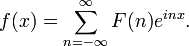
Analysis of periodic functions or functions with limited duration
When ƒ(x) has finite duration (or compact support), a discrete subset of the values of its continuous Fourier transform is sufficient to reconstruct/represent the function ƒ(x) on its support. One such discrete set is obtained by treating the duration of the segment as if it is the period of a periodic function and computing the Fourier coefficients. Putting convergence issues aside, the Fourier series expansion will be a periodic function not the finite-duration function ƒ(x); but one period of the expansion will give the values of ƒ(x) on its support.See Fourier series for more information, including:
- Fourier series expansions for general periods,
- transform properties,
- historical development,
- special cases and generalizations.
Discrete-time Fourier transform (DTFT)
A useful "discrete-time" function can be obtained by sampling a "continuous-time" function, s(t), which produces a sequence, s(nT), for integer values of n and some time-interval T. If information is lost, then only an approximation to the original transform, S(f), can be obtained by looking at one period of the periodic function:
![S_T(f) = \sum_{k=-\infty}^{\infty} S\left(f - \frac{k}{T}\right) \equiv \sum_{n=-\infty}^{\infty} \underbrace{T\cdot s(nT)}_{s[n]} \cdot e^{-i 2\pi f n T},](http://upload.wikimedia.org/math/2/f/9/2f94316f0520418fd281e314b3ad9cde.png)
Applications of the DTFT are not limited to sampled functions. It can be applied to any discrete sequence. See Discrete-time Fourier transform for more information on this and other topics, including:
- the inverse transform
- normalized frequency units
- windowing (finite-length sequences)
- transform properties
- tabulated transforms of specific functions
Discrete Fourier transform (DFT)
![S[k] = \sum_{n=0}^{N-1} s[n] \cdot e^{-i 2 \pi \frac{k}{N} n}](http://upload.wikimedia.org/math/a/a/9/aa9496797b4e12152f9f5b4d76e3824f.png) for all integer values of k.
for all integer values of k.
When s[n] is not periodic, but its non-zero portion has finite duration (N), ST(ƒ) is continuous and finite-valued. But a discrete subset of its values is sufficient to reconstruct/represent the (finite) portion of s[n] that was analyzed. The same discrete set is obtained by treating N as if it is the period of a periodic function and computing the Fourier series coefficients / DFT.
- The inverse transform of S[k] does not produce the finite-length sequence, s[n], when evaluated for all values of n. (It takes the inverse of ST(ƒ) to do that.) The inverse DFT can only reproduce the entire time-domain if the input happens to be periodic (forever). Therefore it is often said that the DFT is a transform for Fourier analysis of finite-domain, discrete-time functions. An alternative viewpoint is that the periodicity is the time-domain consequence of approximating the continuous-domain function, ST(ƒ), with the discrete subset, S[k]. N can be larger than the actual non-zero portion of s[n]. The larger it is, the better the approximation (also known as zero-padding).
See Discrete Fourier transform for much more information, including:
- the inverse transform
- transform properties
- applications
- tabulated transforms of specific functions
| Name | Time domain | Frequency domain | ||
|---|---|---|---|---|
| Domain property | Function property | Domain property | Function property | |
| (Continuous) Fourier transform | Continuous | Aperiodic | Continuous | Aperiodic |
| Discrete-time Fourier transform | Discrete | Aperiodic | Continuous | Periodic (ƒs) |
| Fourier series | Continuous | Periodic (τ) | Discrete | Aperiodic |
| Discrete Fourier transform | Discrete | Periodic (N)[1] | Discrete | Periodic (N) |
Fourier transforms on arbitrary locally compact abelian topological groups
The Fourier variants can also be generalized to Fourier transforms on arbitrary locally compact abelian topological groups, which are studied in harmonic analysis; there, the Fourier transform takes functions on a group to functions on the dual group. This treatment also allows a general formulation of the convolution theorem, which relates Fourier transforms and convolutions. See also the Pontryagin duality for the generalized underpinnings of the Fourier transform.Time-frequency transforms
Time-frequency transforms such as the short-time Fourier transform, wavelet transforms, chirplet transforms, and the fractional Fourier transform try to obtain frequency information from a signal as a function of time (or whatever the independent variable is), although the ability to simultaneously resolve frequency and time is limited by the (mathematical) uncertainty principle.Interpretation in terms of time and frequency
In signal processing, the Fourier transform often takes a time series or a function of continuous time, and maps it into a frequency spectrum. That is, it takes a function from the time domain into the frequency domain; it is a decomposition of a function into sinusoids of different frequencies; in the case of a Fourier series or discrete Fourier transform, the sinusoids are harmonics of the fundamental frequency of the function being analyzed.When the function ƒ is a function of time and represents a physical signal, the transform has a standard interpretation as the frequency spectrum of the signal. The magnitude of the resulting complex-valued function F at frequency ω represents the amplitude of a frequency component whose initial phase is given by the phase of F.
However, it is important to realize that Fourier transforms are not limited to functions of time, and temporal frequencies. They can equally be applied to analyze spatial frequencies, and indeed for nearly any function domain.
How it works (a basic explanation)
To measure the amplitude and phase of a particular frequency component, the transform process multiplies the original function (the one being analyzed) by a sinusoid with the same frequency (called a basis function). If the original function contains a component with the same shape (i.e. same frequency), its shape (but not its amplitude) is effectively squared.- Squaring implies that at every point on the product waveform, the contribution of the matching component to that product is a positive contribution, even though the component might be negative.
- Squaring describes the case where the phases happen to match. What happens more generally is that a constant phase difference produces vectors at every point that are all aimed in the same direction, which is determined by the difference between the two phases. To make that happen actually requires two sinusoidal basis functions, cosine and sine, which are combined into a basis function that is complex-valued (see Complex exponential). The vector analogy refers to the polar coordinate representation.
- Note that if the functions are continuous, rather than sets of discrete points, this step requires integral calculus or numerical integration. But the basic concept is just addition.
See also
- Fourier series
- Bispectrum
- Characteristic function (probability theory)
- Fractional Fourier transform
- Laplace transform
- Least-squares spectral analysis
- Mellin transform
- Number-theoretic transform
- Orthogonal functions
- Pontryagin duality
- Schwartz space
- Spectral density
- Spectral density estimation
- Two-sided Laplace transform
- Wavelet
Notes
- ^ Or N is simply the length of a finite sequence. In either case, the inverse DFT formula produces a periodic function, s[n].
References
- Conte, S. D. & de Boor, Carl (1980), Elementary Numerical Analysis (Third Edition ed.), New York: McGraw Hill, Inc., ISBN 0-07-012447-7
- Evans, Lawrence (1998), Partial Differential Equations, American Mathematical Society
- Edward W. Kamen, Bonnie S. Heck, "Fundamentals of Signals and Systems Using the Web and Matlab", ISBN 0-13-017293-6
- Knuth, Donald E. (1997), The Art of Computer Programming Volume 2: Seminumerical Algorithms (3rd ed.), Section 4.3.3.C: Discrete Fourier transforms, pg.305: Addison-Wesley Professional, ISBN 0201896842
- A. D. Polyanin and A. V. Manzhirov, Handbook of Integral Equations, CRC Press, Boca Raton, 1998. ISBN 0-8493-2876-4
- Rudin, Walter (1990), Fourier Analysis on Groups, Wiley-Interscience, ISBN 047152364X
- Smith, Steven W. (1999). The Scientist and Engineer's Guide to Digital Signal Processing, Second Edition, San Diego, Calif.: California Technical Publishing. ISBN 0-9660176-3-3.
- E. M. Stein, G. Weiss, "Introduction to Fourier Analysis on Euclidean Spaces", Princeton University Press, 1971. ISBN 0-691-08078-X
External links
- Tables of Integral Transforms at EqWorld: The World of Mathematical Equations.
- An Intuitive Explanation of Fourier Theory by Steven Lehar.
- Lectures on Image Processing: A collection of 18 lectures in pdf format from Vanderbilt University. Lecture 6 is on the 1- and 2-D Fourier Transform. Lectures 7-15 make use of it., by Alan Peters


Tidak ada komentar:
Posting Komentar