Jumat, 19 September 2008

Matematika Fisika

Kumpulan Materi Perkuliahan Matematika Fisika dari Pendidikan Fisika, FPMIPA. Universitas Pendidikan Indonesia.

Minggu, 14 September 2008

Mathematical physics

From Wikipedia

and
Arip Nurahman
Department of Physics Education, Faculty of Sciences and Mathematics.
Indonesia University of Education
and
Open Course Ware at Massachusetts Institute of Technology, Cambridge, USA. in Physics

Mathematical physics is the scientific discipline concerned with the interface of mathematics and physics. There is no real consensus about what does or does not constitute mathematical physics. A very typical definition is the one given by the Journal of Mathematical Physics: "the application of mathematics to problems in physics and the development of mathematical methods suitable for such applications and for the formulation of physical theories."^[1]

This definition does, however, not cover the situation where results from physics are used to help prove facts in abstract mathematics which themselves have nothing particular to do with physics. This phenomenon has become increasingly important, with developments from string theory research breaking new ground in mathematics. Eric Zaslow coined the phrase physmatics to describe these developments^[2], although other people would consider them as part of mathematical physics proper.

Important fields of research in mathematical physics include: functional analysis/quantum physics, geometry/general relativity and combinatorics/probability theory/statistical physics. More recently, string theory has managed to make contact with many major branches of mathematics including algebraic geometry, topology, and complex geometry.

· 1 Scope of the subject

· 2 Prominent mathematical physicists

· 3 Mathematically rigorous physics

· 4 Notes

· 5 References

· 6 Bibliographical references

o 6.1 The classics

o 6.2 Textbooks for undergraduate studies

o 6.3 Other specialised subareas

· 7 See also

· 8 External links

Scope of the subject

There are several distinct branches of mathematical physics, and these roughly correspond to particular historical periods. The theory of partial differential equations (and the related areas of variational calculus, Fourier analysis, potential theory, and vector analysis) are perhaps most closely associated with mathematical physics. These were developed intensively from the second half of the eighteenth century (by, for example, D'Alembert, Euler, and Lagrange) until the 1930s. Physical applications of these developments include hydrodynamics, celestial mechanics, elasticity theory, acoustics, thermodynamics, electricity, magnetism, and aerodynamics.

The theory of atomic spectra (and, later, quantum mechanics) developed almost concurrently with the mathematical fields of linear algebra, the spectral theory of operators, and more broadly, functional analysis. These constitute the mathematical basis of another branch of mathematical physics.

The special and general theories of relativity require a rather different type of mathematics. This was group theory: and it played an important role in both quantum field theory and differential geometry. This was, however, gradually supplemented by topology in the mathematical description of cosmological as well as quantum field theory phenomena.

Statistical mechanics forms a separate field, which is closely related with the more mathematical ergodic theory and some parts of probability theory.

The usage of the term 'Mathematical physics' is sometimes idiosyncratic. Certain parts of mathematics that initially arose from the development of physics are not considered parts of mathematical physics, while other closely related fields are. For example, ordinary differential equations and symplectic geometry are generally viewed as purely mathematical disciplines, whereas dynamical systems and Hamiltonian mechanics belong to mathematical physics.

Prominent mathematical physicists

One of the earliest mathematical physicists was the eleventh century Iraqi physicist and mathematician, Ibn al-Haytham [965-1039], known in the West as Alhazen. His conceptions of mathematical models and of the role they play in his theory of sense perception, as seen in his Book of Optics (1021), laid the foundations for mathematical physics.^[3] Other notable mathematical physicists at the time included Abū Rayhān al-Bīrūnī [973-1048] and Al-Khazini [fl. 1115-1130], who introduced algebraic and fine calculation techniques into the fields of statics and dynamics.^[4]

The great seventeenth century English physicist and mathematician, Isaac Newton [1642-1727], developed a wealth of new mathematics (for example, calculus and several numerical methods (most notably Newton's method) to solve problems in physics. Other important mathematical physicists of the seventeenth century included the Dutchman Christiaan Huygens [1629-1695] (famous for suggesting the wave theory of light), and the German Johannes Kepler [1571-1630] (Tycho Brahe's assistant, and discoverer of the equations for planetary motion/orbit).

In the eighteenth century, two of the great innovators of mathematical physics were Swiss: Daniel Bernoulli [1700-1782] (for contributions to fluid dynamics, and vibrating strings), and, more especially, Leonhard Euler [1707-1783], (for his work in variational calculus, dynamics, fluid dynamics, and many other things). Another notable contributor was the Italian-born Frenchman, Joseph-Louis Lagrange [1736-1813] (for his work in mechanics and variational methods).

In the late eighteenth and early nineteenth centuries, important French figures were Pierre-Simon Laplace [1749-1827] (in mathematical astronomy, potential theory, and mechanics) and Siméon Denis Poisson [1781-1840] (who also worked in mechanics and potential theory). In Germany, both Carl Friedrich Gauss [1777-1855] (in magnetism) and Carl Gustav Jacobi [1804-1851] (in the areas of dynamics and canonical transformations) made key contributions to the theoretical foundations of electricity, magnetism, mechanics, and fluid dynamics.

Gauss (along with Euler) is considered by many to be one of the three greatest mathematicians of all time. His contributions to non-Euclidean geometry laid the groundwork for the subsequent development of Riemannian geometry by Bernhard Riemann [1826-1866]. As we shall see later, this work is at the heart of general relativity.

The nineteenth century also saw the Scot, James Clerk Maxwell [1831-1879], win renown for his four equations of electromagnetism, and his countryman, Lord Kelvin [1824-1907] make substantial discoveries in thermodynamics. Among the English physics community, Lord Rayleigh [1842-1919] worked on sound; and George Gabriel Stokes [1819-1903] was a leader in optics and fluid dynamics; while the Irishman William Rowan Hamilton [1805-1865] was noted for his work in dynamics. The German Hermann von Helmholtz [1821-1894] is best remembered for his work in the areas of electromagnetism, waves, fluids, and sound. In the U.S.A., the pioneering work of Josiah Willard Gibbs [1839-1903] became the basis for statistical mechanics. Together, these men laid the foundations of electromagnetic theory, fluid dynamics and statistical mechanics.

The late nineteenth and the early twentieth centuries saw the birth of special relativity. This had been anticipated in the works of the Dutchman, Hendrik Lorentz [1853-1928], with important insights from Jules-Henri Poincaré [1854-1912], but which were brought to full clarity by Albert Einstein [1879-1955]. Einstein then developed the invariant approach further to arrive at the remarkable geometrical approach to gravitational physics embodied in general relativity. This was based on the non-Euclidean geometry created by Gauss and Riemann in the previous century.

Einstein's special relativity replaced the Galilean transformations of space and time with Lorentz transformations in four dimensional Minkowski space-time. His general theory of relativity replaced the flat Euclidean geometry with that of a Riemannian manifold, whose curvature is determined by the distribution of gravitational matter. This replaced Newton's scalar gravitational force by the Riemann curvature tensor.

The other great revolutionary development of the twentieth century has been quantum theory, which emerged from the seminal contributions of Max Planck [1856-1947] (on black body radiation) and Einstein's work on the photoelectric effect. This was, at first, followed by a heuristic framework devised by Arnold Sommerfeld [1868-1951] and Niels Bohr [1885-1962], but this was soon replaced by the quantum mechanics developed by Max Born [1882-1970], Werner Heisenberg [1901-1976], Paul Dirac [1902-1984], Erwin Schrödinger [1887-1961], and Wolfgang Pauli [1900-1958]. This revolutionary theoretical framework is based on a probabilistic interpretation of states, and evolution and measurements in terms of self-adjoint operators on an infinite dimensional vector space (Hilbert space, introduced by David Hilbert [1862-1943]). Paul Dirac, for example, used algebraic constructions to produce a relativistic model for the electron, predicting its magnetic moment and the existence of its antiparticle, the positron.

Later important contributors to twentieth century mathematical physics include Satyendra Nath Bose [1894-1974], Julian Schwinger [1918-1994], Sin-Itiro Tomonaga [1906-1979], Richard Feynman [1918-1988], Freeman Dyson [1923- ], Hideki Yukawa [1907-1981], Roger Penrose [1931- ], Stephen Hawking [1942- ], and Edward Witten [1951- ].

Mathematically rigorous physics

The term 'mathematical' physics is also sometimes used in a special sense, to distinguish research aimed at studying and solving problems inspired by physics within a mathematically rigorous framework. Mathematical physics in this sense covers a very broad area of topics with the common feature that they blend pure mathematics and physics. Although related to theoretical physics, 'mathematical' physics in this sense emphasizes the mathematical rigour of the same type as found in mathematics. On the other hand, theoretical physics emphasizes the links to observations and experimental physics which often requires theoretical physicists (and mathematical physicists in the more general sense) to use heuristic, intuitive, and approximate arguments. Such arguments are not considered rigorous by mathematicians. Arguably, rigorous mathematical physics is closer to mathematics, and theoretical physics is closer to physics.

Such mathematical physicists primarily expand and elucidate physical theories. Because of the required rigor, these researchers often deal with questions that theoretical physicists have considered to already be solved. However, they can sometimes show (but neither commonly nor easily) that the previous solution was incorrect.

The field has concentrated in three main areas: (1) quantum field theory, especially the precise construction of models; (2) statistical mechanics, especially the theory of phase transitions; and (3) nonrelativistic quantum mechanics (Schrödinger operators), including the connections to atomic and molecular physics.

The effort to put physical theories on a mathematically rigorous footing has inspired many mathematical developments. For example, the development of quantum mechanics and some aspects of functional analysis parallel each other in many ways. The mathematical study of quantum statistical mechanics has motivated results in operator algebras. The attempt to construct a rigorous quantum field theory has brought about progress in fields such as representation theory. Use of geometry and topology plays an important role in string theory. The above are just a few examples. An examination of the current research literature would undoubtedly give other such instances.

Notes

^ Definition from the Journal of Mathematical Physics.^[1]
^ Zaslow E.,Physmatics
^ Thiele, Rüdiger (August 2005), "In Memoriam: Matthias Schramm, 1928–2005", Historia Mathematica 32(3): 271–274, doi:10.1016/j.hm.2005.05.002
^ Mariam Rozhanskaya and I. S. Levinova (1996), "Statics", p. 642, in (Morelon & Rashed 1996, pp. 614-642)

References

Rashed, Roshdi & Régis Morelon (1996), Encyclopedia of the History of Arabic Science, vol. 1 & 3, Routledge, ISBN 0415124107
Zalsow, Eric (2005), Physmatics, <http://arxiv.org/abs/physics/0506153>

Bibliographical references

The classics

· Abraham, Ralph & Marsden, Jerrold E. (2008), Foundations of mechanics: a mathematical exposition of classical mechanics with an introduction to the qualitative theory of dynamical systems (2nd ed.), Providence, [RI.]: AMS Chelsea Pub., ISBN 9780821844380

· Arnold, Vladimir I.; Vogtmann, K. & Weinstein, A. (tr.) (1997), Mathematical methods of classical mechanics / [Matematicheskie metody klassicheskoĭ mekhaniki] (2nd ed.), New York, [NY.]: Springer-Verlag, ISBN 0-387-96890-3

· Courant, Richard & Hilbert, David (1989), Methods of mathematical physics / [Methoden der mathematischen Physik], New York, [NY.]: Interscience Publishers

· Glimm, James & Jaffe, Arthur (1987), Quantum physics: a functional integral point of view (2nd ed.), New York, [NY.]: Springer-Verlag, ISBN 0-387-96477-0 (pbk.)

· Haag, Rudolf (1996), Local quantum physics: fields, particles, algebras (2nd rev. & enl. ed.), Berlin, [Germany] ; New York, [NY.]: Springer-Verlag, ISBN 3-540-61049-9 (softcover)

· Hawking, Stephen W. & Ellis, George F. R. (1973), The large scale structure of space-time, Cambridge, [England]: Cambridge University Press, ISBN 0-521-20016-4

· Kato, Tosio (1995), Perturbation theory for linear operators (2nd repr. ed.), Berlin, [Germany]: Springer-Verlag, ISBN 3-540-58661-X

· This is a reprint of the second (1980) edition of this title.

· Margenau, Henry & Murphy, George Moseley (1976), The mathematics of physics and chemistry (2nd repr. ed.), Huntington, [NY.]: R. E. Krieger Pub. Co., ISBN 0-882-75423-8

· This is a reprint of the 1956 second edition.

· Morse, Philip McCord & Feshbach, Herman (1999), Methods of theoretical physics (repr. ed.), Boston, {Mass.]: McGraw Hill, ISBN 0-070-43316-X

· This is a reprint of the original (1953) edition of this title.

· von Neumann, John & Beyer, Robert T. (tr.) (1955), Mathematical foundations of quantum mechanics, Princeton, [NJ.]: Princeton University Press

· Reed, Michael C. & Simon, Barry (1972-1977), Methods of modern mathematical physics (4 vol.), New York. {NY.]: Academic Press, ISBN 0-125-85001-8

· Titchmarsh, Edward Charles (1939), The theory of functions (2nd ed.), London, [England]: Oxford University Press

· This tome was reprinted in 1985.

· Thirring, Walter E. & Harrell, Evans M. (tr.) (1978-1983), A course in mathematical physics / [Lehrbuch der mathematischen Physik] (4 vol.), New York, [NY.]: Springer-Verlag

· Weyl, Hermann & Robertson, H. P. (tr.) (1931), The theory of groups and quantum mechanics / [Gruppentheorie und Quantenmechanik], London, [England]: Methuen & Co.

· Whittaker, Edmund Taylor & Watson, George Neville (1979), A course of modern analysis: an introduction to the general theory of infinite processes and of analytic functions, with an account of the principal transcendental functions (1st AMS ed.), New York, [NY.]: AMS Press, ISBN 0-404-14736-4

Textbooks for undergraduate studies

· Arfken, George B. & Weber, Hans J. (1995), Mathematical methods for physicists (4th ed.), San Diego, [CA.]: Academic Press, ISBN 0-120-59816-7 (pbk.)

· Boas, Mary L. (2006), Mathematical methods in the physical sciences (3rd ed.), Hoboken, [NJ.]: John Wiley & Sons, ISBN 9780471198260

· Butkov, Eugene (1968), Mathematical physics, Reading, [Mass.]: Addison-Wesley

· Jeffreys, Harold & Swirles Jeffreys, Bertha (1956), Methods of mathematical physics (3rd rev. ed.), Cambridge, [England]: Cambridge University Press

· Mathews, Jon & Walker, Robert L. (1970), Mathematical methods of physics (2nd ed.), New York, [NY.]: W. A. Benjamin, ISBN 0-8053-7002-1

· Stakgold, Ivar (c.2000), Boundary value problems of mathematical physics (2 vol.), Philadelphia, [PA.]: Society for Industrial and Applied Mathematics, ISBN 0-898-71456-7 (set : pbk.)

Other specialised subareas

· Aslam, Jamil & Hussain, Faheem (2007), 'Mathematical physics' Proceedings of the 12th Regional Conference, Islamabad, Pakistan, 27 March - 1 April 2006], Singapore: World Scientific, ISBN 978-981-270-591-4, <http://www.worldscibooks.com/physics/6405.html>

· Baez, John C. & Muniain, Javier P. (1994), Gauge fields, knots, and gravity, Singapore ; River Edge, [NJ.]: World Scientific, ISBN 9-810-22034-0 (pbk.)

· Geroch, Robert (1985), Mathematical physics, Chicago, [IL.]: University of Chicago Press, ISBN 0-226-28862-5 (pbk.)

· Polyanin, Andrei D. (2002), Handbook of linear partial differential equations for engineers and scientists, Boca Raton, [FL.]: Chapman & Hall / CRC Press, ISBN 1-584-88299-9

· Polyanin, Alexei D. & Zaitsev, Valentin F. (2004), Handbook of nonlinear partial differential equations, Boca Raton, [FL.]: Chapman & Hall / CRC Press, ISBN 1-584-88355-3

· Szekeres, Peter (2004), A course in modern mathematical physics: groups, Hilbert space and differential geometry, Cambridge, [England] ; New York, [NY.]: Cambridge University Press, ISBN 0-521-53645-6 (pbk.)

External links

v • d • e

Major fields of mathematics

Arithmetic · Logic · Set theory · Category theory · Algebra (elementary – linear – abstract) · Number theory · Analysis · Geometry · Trigonometry · Topology · Dynamical systems · Combinatorics · Game theory · Information theory · Optimization · Computation · Probability · Statistics · Mathematical physics

Retrieved from "http://en.wikipedia.org/wiki/Mathematical_physics"

Categories: Mathematical physics | Mathematical science occupations

Partial Differential Equation

Partial differential equation

From Wikipedia

Arip Nurahman
Department of Physics Education, Faculty of Sciences and Mathematics.
Indonesia University of Education
and
Open Course Ware at Massachusetts Institute of Technology, Cambridge, USA. in Physics

In mathematics, partial differential equations (PDE) are a type of differential equation, i.e., a relation involving an unknown function (or functions) of several independent variables and its (resp. their) partial derivatives with respect to those variables. Partial differential equations are used to formulate, and thus aid the solution of, problems involving functions of several variables; such as the propagation of sound or heat, electrostatics, electrodynamics, fluid flow, elasticity. Interestingly, seemingly distinct physical phenomena may have identical mathematical formulations, and thus be governed by the same underlying dynamic.

Introduction

A relatively simple partial differential equation is

$\frac{\partial}{\partial x}u(x,y)=0\, .$

This relation implies that the values u(x,y) are independent of x. Hence the general solution of this equation is

$u(x,y) = f(y),\,$

where f is an arbitrary function of y. The analogous ordinary differential equation is

$\frac{du}{dx}=0\,$

which has the solution

$u(x) = c,\,$

where c is any constant value (independent of x). These two examples illustrate that general solutions of ordinary differential equations involve arbitrary constants, but solutions of partial differential equations involve arbitrary functions. A solution of a partial differential equation is generally not unique; additional conditions must generally be specified on the boundary of the region where the solution is defined. For instance, in the simple example above, the function

f (y)

can be determined if

u

is specified on the line

x = 0

Existence and uniqueness

Although the issue of the existence and uniqueness of solutions of ordinary differential equations has a very satisfactory answer with the Picard-Lindelöf theorem, that is far from the case for partial differential equations. There is a general theorem (the Cauchy-Kovalevskaya theorem) that states that the Cauchy problem for any partial differential equation that is analytic in the unknown function and its derivatives have a unique analytic solution. Although this result might appear to settle the existence and uniqueness of solutions, there are examples of linear partial differential equations whose coefficients have derivatives of all orders (which are nevertheless not analytic) but which have no solutions at all: see Lewy (1957). Even if the solution of a partial differential equation exists and is unique, it may nevertheless have undesirable properties. The mathematical study of these questions is usually in the more powerful context of weak solutions.

An example of pathological behavior is the sequence of Cauchy problems (depending upon n) for the Laplace equation

$\frac{\part^2 u}{\partial x^2} + \frac{\part^2 u}{\partial y^2}=0,\,$

with initial conditions

$u(x,0) = 0, \,$

$\frac{\partial u}{\partial y}(x,0) = \frac{\sin n x}{n},\,$

where n is an integer. The derivative of u with respect to y approaches 0 uniformly in x as n increases, but the solution is

$u(x,y) = \frac{(\sinh ny)(\sin nx)}{n^2}.\,$

This solution approaches infinity if nx is not an integer multiple of π for any non-zero value of y. The Cauchy problem for the Laplace equation is called ill-posed or not well posed, since the solution does not depend continuously upon the data of the problem. Such ill-posed problems are not usually satisfactory for physical applications.

Notation

In PDEs, it is common to denote partial derivatives using subscripts. That is:

$u_x = {\partial u \over \partial x}$

$u_{xy} = {\part^2 u \over \partial y\, \partial x} = {\partial \over \partial y } \left({\partial u \over \partial x}\right).$

Especially in (mathematical) physics, one often prefers use of del (which in cartesian coordinates is written $\nabla=(\part_x,\part_y,\part_z)\,$ ) for spatial derivatives and a dot $\dot u\,$ for time derivatives, e.g. to write the wave equation (see below) as

$\ddot u=c^2\triangle u.\,$ (math notation)

$\ddot u=c^2\nabla^2u.\,$ (physics notation)

Examples

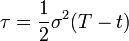
Heat equation in one space dimension

The equation for conduction of heat in one dimension for a homogeneous body has the form

$u_t = \alpha u_{xx} \,$

where u(t,x) is temperature, and α is a positive constant that describes the rate of diffusion. The Cauchy problem for this equation consists in specifying

u (0, x) = f (x)

, where f(x) is an arbitrary function.

General solutions of the heat equation can be found by the method of separation of variables. Some examples appear in the heat equation article. They are examples of Fourier series for periodic f and Fourier transforms for non-periodic f. Using the Fourier transform, a general solution of the heat equation has the form

$u(t,x) = \frac{1}{\sqrt{2\pi}} \int_{-\infty}^{\infty} F(\xi) e^{-\alpha \xi^2 t} e^{i \xi x} d\xi, \,$

where F is an arbitrary function. In order to satisfy the initial condition, F is given by the Fourier transform of f, that is

$F(\xi) = \frac{1}{\sqrt{2\pi}} \int_{-\infty}^{\infty} f(x) e^{-i \xi x}\, dx. \,$

If f represents a very small but intense source of heat, then the preceding integral can be approximated by the delta distribution, multiplied by the strength of the source. For a source whose strength is normalized to 1, the result is

$F(\xi) = \frac{1}{\sqrt{2\pi}}, \,$

and the resulting solution of the heat equation is

$u(t,x) = \frac{1}{2\pi} \int_{-\infty}^{\infty}e^{-\alpha \xi^2 t} e^{i \xi x} d\xi. \,$

This is a Gaussian integral. It may be evaluated to obtain

$u(t,x) = \frac{1}{2\sqrt{\pi \alpha t}} \exp\left(-\frac{x^2}{4 \alpha t} \right). \,$

This result corresponds to a normal probability density for x with mean 0 and variance 2αt. The heat equation and similar diffusion equations are useful tools to study random phenomena.

Wave equation in one spatial dimension

The wave equation is an equation for an unknown function u(t, x) of the form

$u_{tt} = c^2 u_{xx}. \,$

Here u might describe the displacement of a stretched string from equilibrium, or the difference in air pressure in a tube, or the magnitude of an electromagnetic field in a tube, and c is a number that corresponds to the velocity of the wave. The Cauchy problem for this equation consists in prescribing the initial displacement and velocity of a string or other medium:

$u(0,x) = f(x), \,$

$u_t(0,x) = g(x), \,$

where f and g are arbitrary given functions. The solution of this problem is given by d'Alembert's formula:

$u(t,x) = \frac{1}{2} \left[f(x-ct) + f(x+ct)\right] + \frac{1}{2c}\int_{x-ct}^{x+ct} g(y)\, dy. \,$

This formula implies that the solution at (t,x) depends only upon the data on the segment of the initial line that is cut out by the characteristic curves

$x - ct = \hbox{constant,} \quad x + ct = \hbox{constant}, \,$

that are drawn backwards from that point. These curves correspond to signals that propagate with velocity c forward and backward. Conversely, the influence of the data at any given point on the initial line propagates with the finite velocity c: there is no effect outside a triangle through that point whose sides are characteristic curves. This behavior is very different from the solution for the heat equation, where the effect of a point source appears (with small amplitude) instantaneously at every point in space. The solution given above is also valid if t is negative, and the explicit formula shows that the solution depends smoothly upon the data: both the forward and backward Cauchy problems for the wave equation are well-posed.

Spherical waves

Spherical waves are waves whose amplitude depends only upon the radial distance r from a central point source. For such waves, the three-dimensional wave equation takes the form

$u_{tt} = c^2 \left[u_{rr} + \frac{2}{r} u_r \right]. \,$

This is equivalent to

$(ru)_{tt} = c^2 \left[(ru)_{rr} \right],\,$

and hence the quantity ru satisfies the one-dimensional wave equation. Therefore a general solution for spherical waves has the form

$u(t,r) = \frac{1}{r} \left[F(r-ct) + G(r+ct) \right],\,$

where F and G are completely arbitrary functions. Radiation from an antenna corresponds to the case where G is identically zero. Thus the wave form transmitted from an antenna has no distortion in time: the only distorting factor is 1/r. This feature of undistorted propagation of waves is not present if there are two spatial dimensions.

Laplace equation in two dimensions

The Laplace equation for an unknown function of two variables φ has the form

$\varphi_{xx} + \varphi_{yy} = 0.$

Solutions of Laplace's equation are called harmonic functions.

Connection with holomorphic functions

Solutions of the Laplace equation in two dimensions are intimately connected with analytic functions of a complex variable (a.k.a. holomorphic functions): the real and imaginary parts of any analytic function are conjugate harmonic functions: they both satisfy the Laplace equation, and their gradients are orthogonal. If f=u+iv, then the Cauchy-Riemann equations state that

$u_x = v_y, \quad v_x = -u_y,\,$

and it follows that

$u_{xx} + u_{yy} = 0, \quad v_{xx} + v_{yy}=0. \,$

Conversely, given any harmonic function in two dimensions, it is the real part of an analytic function, at least locally. Details are given in Laplace equation.

A typical boundary value problem

A typical problem for Laplace's equation is to find a solution that satisfies arbitrary values on the boundary of a domain. For example, we may seek a harmonic function that takes on the values u(θ) on a circle of radius one. The solution was given by Poisson:

$\varphi(r,\theta) = \frac{1}{2\pi} \int_0^{2\pi} \frac{1-r^2}{1 +r^2 -2r\cos (\theta -\theta')} u(\theta')d\theta'.\,$

Petrovsky (1967, p. 248) shows how this formula can be obtained by summing a Fourier series for φ. If r<1,>u is continuous but not necessarily differentiable. This behavior is typical for solutions of elliptic partial differential equations: the solutions may be much more smooth than the boundary data. This is in contrast to solutions of the wave equation, and more general hyperbolic partial differential equations, which typically have no more derivatives than the data.

Euler-Tricomi equation

The Euler-Tricomi equation is used in the investigation of transonic flow.

$u_{xx} \, =xu_{yy}.$

Advection equation

The advection equation describes the transport of a conserved scalar

ψ

in a velocity field ${\bold u}=(u,v,w)$ . It is:

$\psi_t+(u\psi)_x+(v\psi)_y+(w\psi)_z \, =0.$

If the velocity field is solenoidal (that is, $\nabla\cdot{\bold u}=0$ ), then the equation may be simplified to

$\psi_t+u\psi_x+v\psi_y+w\psi_z \, =0.$

The one dimensional steady flow advection equation

ψ t + u .ψ x = 0

(where

u

is constant) is commonly referred to as the pigpen problem. If

u

is not constant and equal to

ψ

the equation is referred to as Burgers' equation.

Ginzburg-Landau equation

The Ginzburg-Landau equation is used in modelling superconductivity. It is

$iu_t+pu_{xx} +q|u|^2u \, =i\gamma u$

where $p,q\in\mathbb{C}$ and $\gamma\in\mathbb{R}$ are constants and

i

is the imaginary unit.

The Dym equation

The Dym equation is named for Harry Dym and occurs in the study of solitons. It is

$u_t \, = u^3u_{xxx}.$

Initial-boundary value problems

Main article: Boundary value problem

Further information: Examples of boundary value problems

Many problems of Mathematical Physics are formulated as initial-boundary value problems.

Vibrating string

If the string is stretched between two points where x=0 and x=L and u denotes the amplitude of the displacement of the string, then u satisfies the one-dimensional wave equation in the region where 0<x<L and t is unlimited. Since the string is tied down at the ends, u must also satisfy the boundary conditions

$u(t,0)=0, \quad u(t,L)=0, \,$

as well as the initial conditions

$u(0,x)=f(x), \quad u_t(0,x)=g(x). \,$

The method of separation of variables for the wave equation

$u_{tt} = c^2 u_{xx}, \,$

leads to solutions of the form

$u(t,x) = T(t) X(x),\,$

where

$T'' + k^2 c^2 T=0, \quad X'' + k^2 X=0,\,$

where the constant k must be determined. The boundary conditions then imply that X is a multiple of sin kx, and k must have the form

$k= \frac{n\pi}{L}, \,$

where n is an integer. Each term in the sum corresponds to a mode of vibration of the string. The mode with n=1 is called the fundamental mode, and the frequencies of the other modes are all multiples of this frequency. They form the overtone series of the string, and they are the basis for musical acoustics. The initial conditions may then be satisfied by representing f and g as infinite sums of these modes. Wind instruments typically correspond to vibrations of an air column with one end open and one end closed. The corresponding boundary conditions are

$X(0) =0, \quad X'(L) = 0.\,$

The method of separation of variables can also be applied in this case, and it leads to a series of odd overtones.

The general problem of this type is solved in Sturm-Liouville theory.

Vibrating membrane

If a membrane is stretched over a curve C that forms the boundary of a domain D in the plane, its vibrations are governed by the wave equation

$\frac{1}{c^2} u_{tt} = u_{xx} + u_{yy}, \,$

if t>0 and (x,y) is in D. The boundary condition is

u (t, x, y) = 0

(x, y)

is on

C

. The method of separation of variables leads to the form

$u(t,x,y) = T(t) v(x,y),\,$

which in turn must satisfy

$\frac{1}{c^2}T'' +k^2 T=0, \,$

$v_{xx} + v_{yy} + k^2 v =0.\,$

The latter equation is called the Helmholtz Equation. The constant k must be determined in order to allow a non-trivial v to satisfy the boundary condition on C. Such values of k² are called the eigenvalues of the Laplacian in D, and the associated solutions are the eigenfunctions of the Laplacian in D. The Sturm-Liouville theory may be extended to this elliptic eigenvalue problem (Jost, 2002).

There are no generally applicable methods to solve non-linear PDEs. Still, existence and uniqueness results (such as the Cauchy-Kovalevskaya theorem) are often possible, as are proofs of important qualitative and quantitative properties of solutions (getting these results is a major part of analysis). Computational solution to the nonlinear PDEs, the Split-step method, exist for specific equations like nonlinear Schrödinger equation.

Nevertheless, some techniques can be used for several types of equations. The h-principle is the most powerful method to solve underdetermined equations. The Riquier-Janet theory is an effective method for obtaining information about many analytic overdetermined systems.

The method of characteristics (Similarity Transformation method) can be used in some very special cases to solve partial differential equations.

In some cases, a PDE can be solved via perturbation analysis in which the solution is considered to be a correction to an equation with a known solution. Alternatives are numerical analysis techniques from simple finite difference schemes to the more mature multigrid and finite element methods. Many interesting problems in science and engineering are solved in this way using computers, sometimes high performance supercomputers.

Other examples

The Schrödinger equation is a PDE at the heart of non-relativistic quantum mechanics. In the WKB approximation it is the Hamilton-Jacobi equation.

Except for the Dym equation and the Ginzburg-Landau equation, the above equations are linear in the sense that they can be written in the form Au = f for a given linear operator A and a given function f. Other important non-linear equations include the Navier-Stokes equations describing the flow of fluids, and Einstein's field equations of general relativity.

Also see the list of non-linear partial differential equations.

Classification

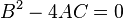
Some linear, second-order partial differential equations can be classified as parabolic, hyperbolic or elliptic. Others such as the Euler-Tricomi equation have different types in different regions. The classification provides a guide to appropriate initial and boundary conditions, and to smoothness of the solutions.

Equations of first order

Main article: First order partial differential equation

Equations of second order

Assuming

u x y = u y x

, the general second-order PDE in two independent variables has the form

$Au_{xx} + Bu_{xy} + Cu_{yy} + \cdots = 0,$

where the coefficients A, B, C etc. may depend upon x and y. This form is analogous to the equation for a conic section:

$Ax^2 + Bxy + Cy^2 + \cdots = 0.$

Just as one classifies conic sections into parabolic, hyperbolic, and elliptic based on the discriminant

B 2 - 4 A C

, the same can be done for a second-order PDE at a given point.

: solutions of elliptic PDEs are as smooth as the coefficients allow, within the interior of the region where the equation and solutions are defined. For example, solutions of Laplace's equation are analytic within the domain where they are defined, but solutions may assume boundary values that are not smooth. The motion of a fluid at subsonic speeds can be approximated with elliptic PDEs, and the Euler-Tricomi equation is elliptic where x<0.
$B^2 - 4AC = 0\,$ : equations that are parabolic at every point can be transformed into a form analogous to the heat equation by a change of independent variables. Solutions smooth out as the transformed time variable increases. The Euler-Tricomi equation has parabolic type on the line where x=0.
$\text{[math]}$ 0 " src="http://upload.wikimedia.org/math/d/6/0/d6020eb939839e531ab6cc27f7ae1f94.png"> : hyperbolic equations retain any discontinuities of functions or derivatives in the initial data. An example is the wave equation. The motion of a fluid at supersonic speeds can be approximated with hyperbolic PDEs, and the Euler-Tricomi equation is hyperbolic where x>0.

If there are n independent variables x₁, x₂ , ..., x_n, a general linear partial differential equation of second order has the form

$L u =\sum_{i=1}^n\sum_{j=1}^n a_{i,j} \frac{\part^2 u}{\partial x_i \partial x_j} \quad \hbox{ plus lower order terms} =0. \,$

The classification depends upon the signature of the eigenvalues of the coefficient matrix.

Elliptic: The eigenvalues are all positive or all negative.
Parabolic : The eigenvalues are all positive or all negative, save one which is zero.
Hyperbolic: There is only one negative eigenvalue and all the rest are positive, or there is only one positive eigenvalue and all the rest are negative.
Ultrahyperbolic: There is more than one positive eigenvalue and more than one negative eigenvalue, and there are no zero eigenvalues. There is only limited theory for ultrahyperbolic equations (Courant and Hilbert, 1962).

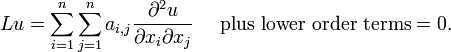
Systems of first-order equations and characteristic surfaces

The classification of partial differential equations can be extended to systems of first-order equations, where the unknown u is now a vector with m components, and the coefficient matrices

A ν

are m by m matrices for $\nu=1, \dots,n$ . The partial differential equation takes the form

$Lu = \sum_{\nu=1}^{n} A_\nu \frac{\partial u}{\partial x_\nu} + B=0, \,$

where the coefficient matrices A_ν and the vector B may depend upon x and u. If a hypersurface S is given in the implicit form

$\varphi(x_1, x_2, \ldots, x_n)=0, \,$

where φ has a non-zero gradient, then S is a characteristic surface for the operator L at a given point if the characteristic form vanishes:

$Q\left(\frac{\part\varphi}{\partial x_1}, \ldots,\frac{\part\varphi}{\partial x_n}\right) =\det\left[\sum_{\nu=1}^nA_\nu \frac{\partial \varphi}{\partial x_\nu}\right]=0.\,$

The geometric interpretation of this condition is as follows: if data for u are prescribed on the surface S, then it may be possible to determine the normal derivative of u on S from the differential equation. If the data on S and the differential equation determine the normal derivative of u on S, then S is non-characteristic. If the data on S and the differential equation do not determine the normal derivative of u on S, then the surface is characteristic, and the differential equation restricts the data on S: the differential equation is internal to S.

A first-order system Lu=0 is elliptic if no surface is characteristic for L: the values of u on S and the differential equation always determine the normal derivative of u on S.
A first-order system is hyperbolic at a point if there is a space-like surface S with normal ξ at that point. This means that, given any non-trivial vector η orthogonal to ξ, and a scalar multiplier λ, the equation

$Q(\lambda \xi + \eta) =0, \,$

has m real roots λ₁, λ₂, ..., λ_m. The system is strictly hyperbolic if these roots are always distinct. The geometrical interpretation of this condition is as follows: the characteristic form Q(ζ)=0 defines a cone (the normal cone) with homogeneous coordinates ζ. In the hyperbolic case, this cone has m sheets, and the axis ζ = λ ξ runs inside these sheets: it does not intersect any of them. But when displaced from the origin by η, this axis intersects every sheet. In the elliptic case, the normal cone has no real sheets.

Equations of mixed type

If a PDE has coefficients which are not constant, it is possible that it will not belong to any of these categories but rather be of mixed type. A simple but important example is the Euler-Tricomi equation

$u_{xx} \, = xu_{yy}$

which is called elliptic-hyperbolic because it is elliptic in the region x <>x > 0, and degenerate parabolic on the line x = 0.

Methods to solve PDEs

Separation of variables

The method of separation of variables will yield particular solutions of a linear PDE on very simple domains such as rectangles that may satisfy initial or boundary conditions.

Change of variable

Often a PDE can be reduced to a simpler form with a known solution by a suitable change of variables. For example the Black–Scholes PDE

$\frac{\partial V}{\partial t} + \frac{1}{2}\sigma^2 S^2\frac{\partial^2 V}{\partial S^2} + rS\frac{\partial V}{\partial S} - rV = 0$

is reducible to the Heat equation

$\frac{\partial u}{\partial \tau} = \frac{\partial^2 u}{\partial x^2}$

by the change of variables (for complete details see Solution of the Black Scholes Equation):

$V(S,t) = K v(x,\tau)\,$

$x = \ln(S/K)\,$

$\tau = \frac{1}{2} \sigma^2 (T - t)$

$v(x,\tau)=exp(-\alpha x-\beta\tau) u(x,\tau).\,$

Method of characteristics

Main article: Method of characteristics

Superposition principle

Because any superposition of solutions of a linear PDE is again a solution, the particular solutions may then be combined to obtain more general solutions.

Fourier series

If the domain is finite or periodic, an infinite sum of solutions such as a Fourier series is appropriate, but an integral of solutions such as a Fourier integral is generally required for infinite domains. The solution for a point source for the heat equation given above is an example for use of a Fourier integral.

References

R. Courant and D. Hilbert, Methods of Mathematical Physics, vol II. Wiley-Interscience, New York, 1962.
L.C. Evans, Partial Differential Equations, American Mathematical Society, Providence, 1998. ISBN 0-8218-0772-2
F. John, Partial Differential Equations, Springer-Verlag, 1982.
J. Jost, Partial Differential Equations, Springer-Verlag, New York, 2002.
Hans Lewy (1957) An example of a smooth linear partial differential equation without solution. Annals of Mathematics, 2nd Series, 66(1),155-158.
I.G. Petrovskii, Partial Differential Equations, W. B. Saunders Co., Philadelphia, 1967.
A. D. Polyanin, Handbook of Linear Partial Differential Equations for Engineers and Scientists, Chapman & Hall/CRC Press, Boca Raton, 2002. ISBN 1-58488-299-9
A. D. Polyanin and V. F. Zaitsev, Handbook of Nonlinear Partial Differential Equations, Chapman & Hall/CRC Press, Boca Raton, 2004. ISBN 1-58488-355-3
A. D. Polyanin, V. F. Zaitsev, and A. Moussiaux, Handbook of First Order Partial Differential Equations, Taylor & Francis, London, 2002. ISBN 0-415-27267-X
D. Zwillinger, Handbook of Differential Equations (3rd edition), Academic Press, Boston, 1997.
Y. Pinchover and J. Rubinstein, An Introduction to Partial Differential Equations, Cambridge University Press, Cambridge, 2005. ISBN 978-0-521-84886-2

External links

Wikimedia Commons has media related to:

Solutions of PDE

Wikibooks has a book on the topic of

Partial Differential Equations

Partial Differential Equations: Exact Solutions at EqWorld: The World of Mathematical Equations.
Partial Differential Equations: Index at EqWorld: The World of Mathematical Equations.
Partial Differential Equations: Methods at EqWorld: The World of Mathematical Equations.
Example problems with solutions at exampleproblems.com
Partial Differential Equations at mathworld.wolfram.com
Dispersive PDE Wiki

Retrieved from "http://en.wikipedia.org/wiki/Partial_differential_equation"

Categories: Multivariable calculus | Partial differential equations

Olimpiade Astro Fisika

Jumat, 19 September 2008

Matematika Fisika

Matematika Fisika

Minggu, 14 September 2008