The sources which I consulted most frequently whilst developing this course are: - Analytical Mechanics:
- G.R. Fowles, Third edition (Holt, Rinehart, & Winston, New York NY, 1977).
- Physics:
- R. Resnick, D. Halliday, and K.S. Krane, Fourth edition, Vol. 1 (John Wiley & Sons, New York NY, 1992).
- Encyclopædia Brittanica:
- Fifteenth edition (Encyclopædia Brittanica, Chicago IL, 1994).
- Physics for scientists and engineers:
- R.A. Serway, and R.J. Beichner, Fifth edition, Vol. 1 (Saunders College Publishing, Orlando FL, 2000).
Classical mechanics is the study of the motion of bodies (including the special case in which bodies remain at rest) in accordance with the general principles first enunciated by Sir Isaac Newton in his Philosophiae Naturalis Principia Mathematica (1687), commonly known as the Principia. Classical mechanics was the first branch of Physics to be discovered, and is the foundation upon which all other branches of Physics are built. Moreover, classical mechanics has many important applications in other areas of science, such as Astronomy (e.g., celestial mechanics), Chemistry (e.g., the dynamics of molecular collisions), Geology (e.g., the propagation of seismic waves, generated by earthquakes, through the Earth's crust), and Engineering (e.g., the equilibrium and stability of structures). Classical mechanics is also of great significance outside the realm of science. After all, the sequence of events leading to the discovery of classical mechanics--starting with the ground-breaking work of Copernicus, continuing with the researches of Galileo, Kepler, and Descartes, and culminating in the monumental achievements of Newton--involved the complete overthrow of the Aristotelian picture of the Universe, which had previously prevailed for more than a millennium, and its replacement by a recognizably modern picture in which humankind no longer played a privileged role.
In our investigation of classical mechanics we shall study many different types of motion, including:
- Translational motion--motion by which a body shifts from one point in space to another (e.g., the motion of a bullet fired from a gun).
- Rotational motion--motion by which an extended body changes orientation, with respect to other bodies in space, without changing position (e.g., the motion of a spinning top).
- Oscillatory motion--motion which continually repeats in time with a fixed period (e.g., the motion of a pendulum in a grandfather clock).
- Circular motion--motion by which a body executes a circular orbit about another fixed body [e.g., the (approximate) motion of the Earth about the Sun].
Of course, these different types of motion can be combined: for instance, the motion of a properly bowled bowling ball consists of a combination of translational and rotational motion, whereas wave propagation is a combination of translational and oscillatory motion. Furthermore, the above mentioned types of motion are not entirely distinct: e.g., circular motion contains elements of both rotational and oscillatory motion. We shall also study statics: i.e., the subdivision of mechanics which is concerned with the forces that act on bodies at rest and in equilibrium. Statics is obviously of great importance in civil engineering: for instance, the principles of statics were used to design the building in which this lecture is taking place, so as to ensure that it does not collapse.
The first principle of any exact science is measurement. In mechanics there are three fundamental quantities which are subject to measurement: - Intervals in space: i.e., lengths.
- Quantities of inertia, or mass, possessed by various bodies.
- Intervals in time.
Any other type of measurement in mechanics can be reduced to some combination of measurements of these three quantities. Each of the three fundamental quantities--length, mass, and time--is measured with respect to some convenient standard. The system of units currently used by all scientists, and most engineers, is called the mks system--after the first initials of the names of the units of length, mass, and time, respectively, in this system: i.e., the meter, the kilogram, and the second.
The mks unit of length is the meter (symbol m), which was formerly the distance between two scratches on a platinum-iridium alloy bar kept at the International Bureau of Metric Standard in Sèvres, France, but is now defined as the distance occupied by  wavelengths of light of the orange-red spectral line of the isotope Krypton 86 in vacuum.
The mks unit of mass is the kilogram (symbol kg), which is defined as the mass of a platinum-iridium alloy cylinder kept at the International Bureau of Metric Standard in Sèvres, France.
The mks unit of time is the second (symbol s), which was formerly defined in terms of the Earth's rotation, but is now defined as the time for  oscillations associated with the transition between the two hyperfine levels of the ground state of the isotope Cesium 133.
In addition to the three fundamental quantities, classical mechanics also deals with derived quantities, such as velocity, acceleration, momentum, angular momentum, etc. Each of these derived quantities can be reduced to some particular combination of length, mass, and time. The mks units of these derived quantities are, therefore, the corresponding combinations of the mks units of length, mass, and time. For instance, a velocity can be reduced to a length divided by a time. Hence, the mks units of velocity are meters per second:
![\begin{displaymath}[v]= \frac{[L]}{[T]} = {\rm m s^{-1}}. \end{displaymath}](http://farside.ph.utexas.edu/teaching/301/lectures/img16.png) | (1) |
Here,  stands for a velocity,
  for a length, and
  for a time, whereas the operator
 ![$[\cdots]$](http://farside.ph.utexas.edu/teaching/301/lectures/img19.png) represents the units, or dimensions, of the quantity contained within the brackets. Momentum can be reduced to a mass times a velocity. Hence, the mks units of momentum are kilogram-meters per second:
represents the units, or dimensions, of the quantity contained within the brackets. Momentum can be reduced to a mass times a velocity. Hence, the mks units of momentum are kilogram-meters per second:
![\begin{displaymath}[p]= [M][v] = \frac{[M][L]}{[T]} = {\rm kg m s^{-1}}. \end{displaymath}](http://farside.ph.utexas.edu/teaching/301/lectures/img20.png) | (2) |
Here,  stands for a momentum, and
  for a mass. In this manner, the mks units of all derived quantities appearing in classical dynamics can easily be obtained.
mks units are specifically designed to conveniently describe those motions which occur in everyday life. Unfortunately, mks units tend to become rather unwieldy when dealing with motions on very small scales (e.g., the motions of molecules) or very large scales (e.g., the motion of stars in the Galaxy). In order to help cope with this problem, a set of standard prefixes has been devised, which allow the mks units of length, mass, and time to be modified so as to deal more easily with very small and very large quantities: these prefixes are specified in Tab. 1. Thus, a kilometer (km) represents  m, a nanometer (nm) represents
  m, and a femtosecond (fs) represents
  s. The standard prefixes can also be used to modify the units of derived quantities.
Table 1: Standard prefixes | Factor | Prefix | Symbol | Factor | Prefix | Symbol |  | exa- | E |  | deci- | d |  | peta- | P |  | centi- | c |  | tera- | T |  | milli- | m |  | giga- | G |  | micro- |  |  | mega- | M | | nano- | n |  | kilo- | k |  | pico- | p |  | hecto- | h | | femto- | f |  | deka- | da |  | atto- | a | |
The mks system is not the only system of units in existence. Unfortunately, the obsolete cgs (centimeter-gram-second) system and the even more obsolete fps (foot-pound-second) system are still in use today, although their continued employment is now strongly discouraged in science and engineering (except in the US!). Conversion between different systems of units is, in principle, perfectly straightforward, but, in practice, a frequent source of error. Witness, for example, the recent loss of the Mars Climate Orbiter because the engineers who designed its rocket engine used fps units whereas the NASA mission controllers employed mks units. Table 2 specifies the various conversion factors between mks, cgs, and fps units. Note that, rather confusingly (unless you are an engineer in the US!), a pound is a unit of force, rather than mass. Additional non-standard units of length include the inch (  ), the yard (
  ), and the mile (
  ). Additional non-standard units of mass include the ton (in the US,
  ; in the UK,
  ), and the metric ton (
  ). Finally, additional non-standard units of time include the minute (
  ), the hour (
  ), the day (
  ), and the year (
  ).
).
Table 2: Conversion factors | 1cm |  | m | | 1g | | kg | | 1ft | |  m m | | 1lb | |  N N | | 1slug | |  kg kg | |
In this course, you are expected to perform calculations to a relative accuracy of 1%: i.e., to three significant figures. Since rounding errors tend to accumulate during lengthy calculations, the easiest way in which to achieve this accuracy is to perform all intermediate calculations to four significant figures, and then to round the final result down to three significant figures. If one of the quantities in your calculation turns out to the the small difference between two much larger numbers, then you may need to keep more than four significant figures. Incidentally, you are strongly urged to use scientific notation in all of your calculations: the use of non-scientific notation is generally a major source of error in this course. If your calculators are capable of operating in a mode in which all numbers (not just very small or very large numbers) are displayed in scientific form then you are advised to perform your calculations in this mode. As we have already mentioned, length, mass, and time are three fundamentally different quantities which are measured in three completely independent units. It, therefore, makes no sense for a prospective law of physics to express an equality between (say) a length and a mass. In other words, the example law  | (3) |
where  is a mass and
  is a length, cannot possibly be correct. One easy way of seeing that Eq. (3) is invalid (as a law of physics), is to note that this equation is dependent on the adopted system of units: i.e., if
  in mks units, then
  in fps units, because the conversion factors which must be applied to the left- and right-hand sides differ. Physicists hold very strongly to the assumption that the laws of physics possess objective reality: in other words, the laws of physics are the same for all observers. One immediate consequence of this assumption is that a law of physics must take the same form in all possible systems of units that a prospective observer might choose to employ. The only way in which this can be the case is if all laws of physics are dimensionally consistent: i.e., the quantities on the left- and right-hand sides of the equality sign in any given law of physics must have the same dimensions (i.e., the same combinations of length, mass, and time). A dimensionally consistent equation naturally takes the same form in all possible systems of units, since the same conversion factors are applied to both sides of the equation when transforming from one system to another.
 As an example, let us consider what is probably the most famous equation in physics:
 | (4) |
Here,  is the energy of a body, is its mass, and
  is the velocity of light in vacuum. The dimensions of energy are
 ![$[M][L^2]/[T^2]$](http://farside.ph.utexas.edu/teaching/301/lectures/img61.png) , and the dimensions of velocity are
, and the dimensions of velocity are ![$[L]/[T]$](http://farside.ph.utexas.edu/teaching/301/lectures/img62.png) . Hence, the dimensions of the left-hand side are , whereas the dimensions of the right-hand side are
. Hence, the dimensions of the left-hand side are , whereas the dimensions of the right-hand side are ![$[M] ([L]/[T])^2= [M][L^2]/[T^2]$](http://farside.ph.utexas.edu/teaching/301/lectures/img63.png) . It follows that Eq. (4) is indeed dimensionally consistent. Thus,
. It follows that Eq. (4) is indeed dimensionally consistent. Thus,  holds good in mks units, in cgs units, in fps units, and in any other sensible set of units. Had Einstein proposed
  , or
, or  , then his error would have been immediately apparent to other physicists, since these prospective laws are not dimensionally consistent. In fact, represents the only simple, dimensionally consistent way of combining an energy, a mass, and the velocity of light in a law of physics.
 The last comment leads naturally to the subject of dimensional analysis: i.e., the use of the idea of dimensional consistency to guess the forms of simple laws of physics. It should be noted that dimensional analysis is of fairly limited applicability, and is a poor substitute for analysis employing the actual laws of physics; nevertheless, it is occasionally useful. Suppose that a special effects studio wants to film a scene in which the Leaning Tower of Pisa topples to the ground. In order to achieve this, the studio might make a scale model of the tower, which is (say) 1m tall, and then film the model falling over. The only problem is that the resulting footage would look completely unrealistic, because the model tower would fall over too quickly. The studio could easily fix this problem by slowing the film down. The question is by what factor should the film be slowed down in order to make it look realistic?
Figure 1: The Leaning Tower of Pisa 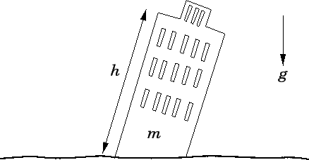 |
Although, at this stage, we do not know how to apply the laws of physics to the problem of a tower falling over, we can, at least, make some educated guesses as to what factors the time  required for this process to occur depends on. In fact, it seems reasonable to suppose that depends principally on the mass of the tower, , the height of the tower,
  , and the acceleration due to gravity,
  . See Fig. 1. In other words,
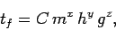 | (5) |
where  is a dimensionless constant, and
  ,
,  , and
, and  are unknown exponents. The exponents , , and can be determined by the requirement that the above equation be dimensionally consistent. Incidentally, the dimensions of an acceleration are
 ![$[L]/[T^2]$](http://farside.ph.utexas.edu/teaching/301/lectures/img74.png) . Hence, equating the dimensions of both sides of Eq. (5), we obtain
. Hence, equating the dimensions of both sides of Eq. (5), we obtain ![\begin{displaymath}[T]= [M]^x [L]^y \left(\frac{[L]}{[T^2]}\right)^z. \end{displaymath}](http://farside.ph.utexas.edu/teaching/301/lectures/img75.png) | (6) |
We can now compare the exponents of ![$[L]$](http://farside.ph.utexas.edu/teaching/301/lectures/img76.png) ,
, ![$[M]$](http://farside.ph.utexas.edu/teaching/301/lectures/img77.png) , and
, and ![$[T]$](http://farside.ph.utexas.edu/teaching/301/lectures/img78.png) on either side of the above expression: these exponents must all match in order for Eq. (5) to be dimensionally consistent. Thus, It immediately follows that
on either side of the above expression: these exponents must all match in order for Eq. (5) to be dimensionally consistent. Thus, It immediately follows that  ,
,  , and
, and  . Hence,
  | (10) |
Now, the actual tower of Pisa is approximately 100m tall. It follows that since  ( is the same for both the real and the model tower) then the 1m high model tower falls over a factor of
  times faster than the real tower. Thus, the film must be slowed down by a factor 10 in order to make it look realistic.
Question: Farmer Jones has recently brought a 40 acre field and wishes to replace the fence surrounding it. Given that the field is square, what length of fencing (in meters) should Farmer Jones purchase? Incidentally, 1 acre equals 43,560 square feet.
Answer: If 1 acre equals 43,560  and 1 ft equals
  (see Tab. 2) then Thus, the area of the field in mks units is Now, a square field with sides of length has an area
  and a circumference
  . Hence,
  . It follows that the length of the fence is Question: The recommended tire pressure in a Honda Civic is 28 psi (pounds per square inch). What is this pressure in atmospheres (1 atmosphere is
  )?
)?
Answer: First, 28 pounds per square inch is the same as  pounds per square foot (the standard fps unit of pressure). Now, 1 pound equals Newtons (the standard SI unit of force), and 1 foot equals m (see Tab. 2). Hence, It follows that 28 psi is equivalent to
  atmospheres.
Question: The speed of sound in a gas might plausibly depend on the pressure , the density  , and the volume
  of the gas. Use dimensional analysis to determine the exponents , , and in the formula where is a dimensionless constant. Incidentally, the mks units of pressure are kilograms per meter per second squared.
Answer: Equating the dimensions of both sides of the above equation, we obtain A comparison of the exponents of , , and on either side of the above expression yields The third equation immediately gives  ; the second equation then yields
  ; finally, the first equation gives
  . Hence,
Added & Edited By:
Arip Nurahman
&
Kawan-kawan
Pendidikan Fisika, FPMIPA, Universitas Pendidikan Indonesia
&
Follower Open Course Ware at MIT-Harvard University, Cambridge. USA.
Terima Kasih Semoga Bermanfaat


![\begin{displaymath} \frac{[L]}{[T]} = \left(\frac{[M]}{[T^2][L]}\right)^x\left( \frac{[M]}{[L^3]}\right)^y [L^3]^z. \end{displaymath}](http://farside.ph.utexas.edu/teaching/301/lectures/img106.png)


