Olimpiade Astro Fisika: Gelombang dan Optik

Gelombang Elektromagnetik

Merupakan Kumpulan Materi Kuliah Gelombang dan Optik

Gelombang Optik

4 SKS

Dosen:

1. Dr. Andhy Setiawan, S.Pd., M.Si.

2. Lina Aviyanti, S.Pd., M.Si.

Sumber Buku:

Drs. Taufik Ramlan Ramalis, M.Si.

Siapakah Cristiano Ronaldo? Atau, siapakah vokalis band Peter Pan? Jika kamu dihadapkan pada pertanyaan semacam itu dapat dipastikan kamu bisa menjawabnya, bukan? Siapa yang tidak kenal CR7 (sebutan buat Cristiano Ronaldo) atau Ariel Peter Pan? Walaupun kamu tidak pernah bertemu secara langsung dengan keduanya, kamu pasti kenal dengan mereka, ya kan? Kok bisa ya! Walaupun kamu tidak pernah bertemu dengan mereka kamu pasti sering melihat mereka melalui TV, bukan begitu? Sekarang, apa yang membuat kamu bisa menonton TV untuk melihat pertandingan sepak bola yang sedang berlangsung di tempat lain yang sangat jauh? Tahukah kamu prinsip dan konsep apa yang melandasi teknologi dan fenomena ini?

Saat ini hampir semua orang memiliki peralatan yang satu ini. Dia begitu kecil yang bisa dengan nyaman diletakkan di dalam saku, namun dianggap memiliki fungsi yang sangat besar terutama untuk berkomunikasi. Ya, benda itu adalah sebuah ponsel (telepon seluler). Saat ini ponsel tidak hanya digunakan untuk menelpon saja tetapi juga untuk fungsi lain seperti mengirim dan menerima pesan singkat (sms), mendengarkan musik, atau mengambil foto. Bagaimana perangkat ponsel dapat terhubung dengan perangkat ponsel yang lain padahal mereka saling berjauhan?

Konsep yang bisa menjelaskan fenomena ini adalah konsep gelombang elektromagnetik. Dan, konsep gelombang elektromagnetik ternyata sangat luas tidak hanya berkaitan dengan TV atau ponsel saja, melainkan banyak aplikasi lain yang bisa sering kita temukan sehari-hari di sekitar kita. Aplikasi tersebut meliputi microwave, radio, radar, atau sinar-x.

The electromagnetic Wave Equation

The electromagnetic wave equation is a second-order partial differential equation that describes the propagation of electromagnetic waves through a medium or in a vacuum. Thehomogeneous form of the equation, written in terms of either the electric field E or the magnetic field B, takes the form:

$\Bigg(\nabla^2$ $- { \mu\epsilon } {\partial^2 \over \partial t^2} \bigg) \mathbf{E}\ \ = \ \ 0$

$\Bigg(\nabla^2$ $- { \mu\epsilon } {\partial^2 \over \partial t^2} \bigg) \mathbf{B}\ \ = \ \ 0$

where c is the speed of light in the medium, and $\nabla^2$ is the Laplace operator. In a vacuum, c = c₀ = 299,792,458 meters per second, which is the speed of light in free space.^[1] The electromagnetic wave equation derives from Maxwell's equations. It should also be noted that in most older literature, B is called the magnetic flux density or magnetic induction.

The origin of the electromagnetic wave equation

Conservation of charge

Conservation of charge requires that the time rate of change of the total charge enclosed within a volume V must equal the net current flowing into the surface S enclosing the volume:

$\oint \limits_S \mathbf{j} \cdot d \mathbf{A} = - {d \over d t} \int \limits_V \rho \cdot dV$

where j is the current density (in amperes per square meter) flowing through the surface and ρ is the charge density (in coulombs per cubic meter) at each point in the volume.

From the divergence theorem, this relationship can be converted from integral form to differential form:

$\nabla \cdot \mathbf{j} = - { \partial \rho \over \partial t}$

Ampère's circuital law prior to Maxwell's correction

In its original form, Ampère's circuital law relates the magnetic field B to the current density j:

$\oint \limits_C \mathbf{B} \cdot d \mathbf{l} = \iint \limits_S \mu \mathbf{j} \cdot d \mathbf{A}$

where S is an open surface terminated in the curve C. This integral form can be converted to differential form, using Stokes' theorem:

$\nabla \times \mathbf{B} = \mu_0 \mathbf{j}$

Inconsistency between Ampère's circuital law and the law of conservation of charge

Taking the divergence of both sides of Ampère's circuital law gives:

$\nabla \cdot ( \nabla \times \mathbf{B} ) = \nabla \cdot \mu_0 \mathbf{j}$

The divergence of the curl of any vector field, including the magnetic field B, is always equal to zero:

$\nabla \cdot ( \nabla \times \mathbf{B}) = 0$

Combining these two equations implies that

$\nabla \cdot \mu_0 \mathbf{j} = 0$

Because $\ \mu_0$ is nonzero constant, it follows that

$\nabla \cdot \mathbf{j} = 0$

However, the law of conservation of charge tells that

$\nabla \cdot \mathbf{j} = - { \partial \rho \over \partial t }$

Hence, as in the case of Kirchhoff's circuit laws, Ampère's circuital law would appear only to hold in situations involving constant charge density. This would rule out the situation that occurs in the plates of a charging or a discharging capacitor.

Maxwell's correction to Ampère's circuital law

Maxwell conceived of displacement current in connection with linear polarization of a dielectric medium. The concept has since been extended to apply to the vacuum. The justification of this virtual extension of displacement current is as follows:

Gauss's law in integral form states:

$\oint \limits_S \mathbf{E} \cdot d \mathbf{A} = \frac{1}{\varepsilon_0} \int \limits_V \rho \cdot dV$

where S is a closed surface enclosing the volume V. This integral form can be converted to differential form using the divergence theorem:

$\nabla \cdot \varepsilon_0 \mathbf{E} = \rho$

Taking the time derivative of both sides and reversing the order of differentiation on the left-hand side gives:

$\nabla \cdot \varepsilon_0 { \partial\mathbf{E} \over \partial t } = { \partial\rho \over \partial t }$

This last result, along with Ampère's circuital law and the conservation of charge equation, suggests that there are actually two origins of the magnetic field: the current density j, as Ampère had already established, and the so-called displacement current:

${\partial\mathbf{D} \over \partial t } = \varepsilon_0 { \partial\mathbf{E} \over \partial t }$

So the corrected form of Ampère's circuital law becomes:

$\nabla \times \mathbf{B} = \mu_0 \mathbf{j} + \mu_0 \varepsilon_0 { \partial\mathbf{E} \over \partial t }$

Maxwell's hypothesis that light is an electromagnetic wave

A postcard from Maxwell toPeter Tait.

In his 1864 paper entitled A Dynamical Theory of the Electromagnetic Field, Maxwell utilized the correction to Ampère's circuital law that he had made in part III of his 1861 paper On Physical Lines of Force. In PART VI of his 1864 paper which is entitled 'ELECTROMAGNETIC THEORY OF LIGHT'^[2], Maxwell combined displacement current with some of the other equations of electromagnetism and he obtained a wave equation with a speed equal to the speed of light. He commented:

The agreement of the results seems to show that light and magnetism are affections of the same substance, and that light is an electromagnetic disturbance propagated through the field according to electromagnetic laws.^[3]

Maxwell's derivation of the electromagnetic wave equation has been replaced in modern physics by a much less cumbersome method involving combining the corrected version of Ampère's circuital law with Faraday's law of induction.

To obtain the electromagnetic wave equation in a vacuum using the modern method, we begin with the modern 'Heaviside' form of Maxwell's equations. In a vacuum and charge free space, these equations are:

$\begin{align} \nabla \cdot \mathbf{E} \;&=\; 0\\ \nabla \times \mathbf{E} \;&=\; -\frac{\partial \mathbf{B}} {\partial t}\\ \nabla \cdot \mathbf{B} \;&=\; 0\\ \nabla \times \mathbf{B} \;&=\; \mu_0 \varepsilon_0 \frac{ \partial \mathbf{E}} {\partial t}\\ \end{align}$

Taking the curl of the curl equations gives:

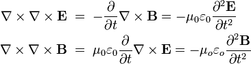
$\begin{align} \nabla \times \nabla \times \mathbf{E} \;&=\; -\frac{\partial } {\partial t} \nabla \times \mathbf{B} = -\mu_0 \varepsilon_0 \frac{\partial^2 \mathbf{E} } {\partial t^2}\\ \nabla \times \nabla \times \mathbf{B} \;&=\; \mu_0 \varepsilon_0 \frac{\partial } {\partial t} \nabla \times \mathbf{E} = -\mu_o \varepsilon_o \frac{\partial^2 \mathbf{B}}{\partial t^2} \end{align}$

By using the vector identity

$\nabla \times \left( \nabla \times \mathbf{V} \right) = \nabla \left( \nabla \cdot \mathbf{V} \right) - \nabla^2 \mathbf{V}$

where $\mathbf{V}$ is any vector function of space, it turns into the wave equations:

$\begin{align} {\partial^2 \mathbf{E} \over \partial t^2} - {c_0}^2 \cdot \nabla^2 \mathbf{E} \;&=\; 0\\ {\partial^2 \mathbf{B} \over \partial t^2} - {c_0}^2 \cdot \nabla^2 \mathbf{B} \;&=\; 0 \end{align}$

where $\scriptstyle c_0 = { 1 \over \sqrt{ \mu_0 \varepsilon_0 } } \,=\, 2.99792458 \times 10^8$ m/s is the speed of light in free space.

Covariant form of the homogeneous wave equation

Time dilation in transversal motion. The requirement that the speed of light is constant in every inertial reference frame leads to the theory of Special Relativity

These relativistic equations can be written in contravariant form as

$\ \Box^2 A^{\mu} = 0$

where the electromagnetic four-potential is

$A^{\mu}=(\varphi, \mathbf{A} c)$

with the Lorenz gauge condition:

$\partial_{\mu} A^{\mu} = 0\,$ .

Where

$\Box^2 = \nabla^2 - { 1 \over c^2} \frac{\partial^2}{\partial t^2}$ is the d'Alembertian operator. (The square box is not a typographical error; it is the correct symbol for this operator.)

Homogeneous wave equation in curved spacetime

Main article: Maxwell's equations in curved spacetime

The electromagnetic wave equation is modified in two ways, the derivative is replaced with the covariant derivative and a new term that depends on the curvature appears.

$-{A^{\alpha ; \beta}}_{; \beta} + {R^{\alpha}}_{\beta} A^{\beta} = 0$

where $\scriptstyle {R^\alpha}_\beta$ is the Ricci curvature tensor and the semicolon indicates covariant differentiation.

The generalization of the Lorenz gauge condition in curved spacetime is assumed:

${A^\mu}_{; \mu} = 0$ .

Inhomogeneous electromagnetic wave equation

Main article: Inhomogeneous electromagnetic wave equation

Localized time-varying charge and current densities can act as sources of electromagnetic waves in a vacuum. Maxwell's equations can be written in the form of a wave equation with sources. The addition of sources to the wave equations makes the partial differential equations inhomogeneous.

[edit]Solutions to the homogeneous electromagnetic wave equation

Main article: Wave equation

The general solution to the electromagnetic wave equation is a linear superposition of waves of the form

$\mathbf{E}( \mathbf{r}, t ) = g(\phi( \mathbf{r}, t )) = g( \omega t - \mathbf{k} \cdot \mathbf{r} )$

and

$\mathbf{B}( \mathbf{r}, t ) = g(\phi( \mathbf{r}, t )) = g( \omega t - \mathbf{k} \cdot \mathbf{r} )$

for virtually any well-behaved function g of dimensionless argument φ, where

$\scriptstyle\omega$ is the angular frequency (in radians per second), and

$\scriptstyle\mathbf{k} \,=\, ( k_x, \,k_y, \,k_z)$ is the wave vector (in radians per meter).

Although the function g can be and often is a monochromatic sine wave, it does not have to be sinusoidal, or even periodic. In practice, g cannot have infinite periodicity because any real electromagnetic wave must always have a finite extent in time and space. As a result, and based on the theory of Fourier decomposition, a real wave must consist of the superposition of an infinite set of sinusoidal frequencies.

In addition, for a valid solution, the wave vector and the angular frequency are not independent; they must adhere to the dispersion relation:

$k = | \mathbf{k} | = { \omega \over c } = { 2 \pi \over \lambda }$

where k is the wavenumber and λ is the wavelength.

Monochromatic, sinusoidal steady-state

The simplest set of solutions to the wave equation result from assuming sinusoidal waveforms of a single frequency in separable form:

$\mathbf{E} ( \mathbf{r}, t ) = \mathrm {Re} \{ \mathbf{E} (\mathbf{r} ) e^{ i \omega t } \}$

where

$\scriptstyle i$ is the imaginary unit,
$\scriptstyle \omega \,=\, 2 \pi f$ is the angular frequency in radians per second,
$\scriptstyle f$ is the frequency in hertz, and
$\scriptstyle e^{i \omega t} \,=\, \cos(\omega t) + i \sin(\omega t) \,$ is Euler's formula.

Plane wave solutions

Main article: Sinusoidal plane-wave solutions of the electromagnetic wave equation

Consider a plane defined by a unit normal vector

$\mathbf{n} = { \mathbf{k} \over k }$ .

Then planar traveling wave solutions of the wave equations are

$\mathbf{E}(\mathbf{r}) = E_0 e^{ -i \mathbf{k} \cdot \mathbf{r} }$

and

$\mathbf{B}(\mathbf{r}) = B_0 e^{ -i \mathbf{k} \cdot \mathbf{r} }$

where

$\scriptstyle\mathbf{r} \,=\, (x, \,y, \,z)$ is the position vector (in meters).

These solutions represent planar waves traveling in the direction of the normal vector $\scriptstyle\mathbf{n}$ . If we define the z direction as the direction of $\scriptstyle\mathbf{n}$ and the x direction as the direction of $\scriptstyle\mathbf{E}$ , then by Faraday's Law the magnetic field lies in the y direction and is related to the electric field by the relation $\scriptstyle c^2{\partial B \over \partial z} \,=\, {\partial E \over \partial t}$ . Because the divergence of the electric and magnetic fields are zero, there are no fields in the direction of propagation.

This solution is the linearly polarized solution of the wave equations. There are also circularly polarized solutions in which the fields rotate about the normal vector.

Spectral decomposition

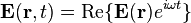
Because of the linearity of Maxwell's equations in a vacuum, solutions can be decomposed into a superposition of sinusoids. This is the basis for the Fourier transform method for the solution of differential equations. The sinusoidal solution to the electromagnetic wave equation takes the form

Electromagnetic spectrum illustration.

$\mathbf{E} ( \mathbf{r}, t ) = \mathbf{E}_0 \cos( \omega t - \mathbf{k} \cdot \mathbf{r} + \phi_0 )$

and

$\mathbf{B} ( \mathbf{r}, t ) = \mathbf{B}_0 \cos( \omega t - \mathbf{k} \cdot \mathbf{r} + \phi_0 )$

where

$\scriptstyle t$ is time (in seconds),

$\scriptstyle \omega$ is the angular frequency (in radians per second),

$\scriptstyle \mathbf{k} \,=\, ( k_x, \,k_y, \,k_z)$ is the wave vector (in radians per meter), and

$\scriptstyle \phi_0$ is the phase angle (in radians).

The wave vector is related to the angular frequency by

$k = | \mathbf{k} | = { \omega \over c } = { 2 \pi \over \lambda }$

where k is the wavenumber and λ is the wavelength.

The electromagnetic spectrum is a plot of the field magnitudes (or energies) as a function of wavelength.

Notes

^ Current practice is to use c₀ to denote the speed of light in vacuum according to ISO 31. In the original Recommendation of 1983, the symbol c was used for this purpose. SeeNIST Special Publication 330, Appendix 2, p. 45
^ Maxwell 1864, page 497.
^ See Maxwell 1864, page 499.

Oleh

Arip Nurahman

Kawan-kawan

Pendidikan Fisika, FPMIPA, Universitas Pendidikan Indonesia

Follower Open Course Ware at MIT-Harvard University, Cambridge. U.S.A.

Terima Kasih, Semoga Bermanfaat

Olimpiade Astro Fisika

Kamis, 05 Februari 2009

Gelombang dan Optik

The origin of the electromagnetic wave equation

Conservation of charge

Ampère's circuital law prior to Maxwell's correction

Inconsistency between Ampère's circuital law and the law of conservation of charge

Maxwell's correction to Ampère's circuital law

Maxwell's hypothesis that light is an electromagnetic wave

Covariant form of the homogeneous wave equation

Homogeneous wave equation in curved spacetime

Inhomogeneous electromagnetic wave equation

[edit]Solutions to the homogeneous electromagnetic wave equation

Monochromatic, sinusoidal steady-state

Plane wave solutions

Spectral decomposition

Other solutions

See also

Theory and Experiment

Applications

Notes

Tidak ada komentar:

International Olympiad on Astronomy and Astrophysics

Mengenai Saya

Kami Terinspirasi

Observatorium Bosscha

Sahabat Team Olimpiade Astro Fisika

Arsip Blog