
Gelombang Optik
4 SKS
Dosen:
1. Dr. Andhy Setiawan, S.Pd., M.Si.
2. Lina Aviyanti, S.Pd., M.Si.
Sumber Buku:
Drs. Taufik Ramlan Ramalis, M.Si.
1. Osilasi Harmonis
a. Pendahuluan
Dunia kita ini penuh dengan benda-benda yang bergerak. Gerak-gerak tersebut dapat kita kelompokkan menjadi dua, yaitu gerak disekitar suatu tempat, dan gerak yang berpindah dari suatu tempat ke tempat lain.
Osilasi adalah variasi periodik - umumnya terhadap waktu - dari suatu hasil pengukuran, contohnya pada ayunan bandul. Istilah vibrasi sering digunakan sebagai sinonim osilasi, walaupun sebenarnya vibrasi merujuk pada jenis spesifik osilasi, yaitu osilasi mekanis. Osilasi tidak hanya terjadi pada suatu sistem fisik, tapi bisa juga pada sistem biologi dan bahkan dalam masyarakat. Osilasi terbagi menjadi 2 yaitu osilasi harmonis sederhana dan osilasi harmonis kompleks. Dalam osilasi harmonis sederhana terdapat gerak harmonis sederhana.
Gerak Harmonik Sederhana
Gerak Harmonik Sederhana (GHS) adalah gerak periodik dengan lintasan yang ditempuh selalu sama (tetap). Gerak Harmonik Sederhana mempunyai persamaan gerak dalam bentuk sinusoidal dan digunakan untuk menganalisis suatu gerak periodik tertentu. Gerak periodik adalah gerak berulang atau berosilasi melalui titik setimbang dalam interval waktu tetap. Gerak Harmonik Sederhana dapat dibedakan menjadi 2 bagian, yaitu :
- Gerak Harmonik Sederhana (GHS) Linier, misalnya penghisap dalam silinder gas, gerak osilasi air raksa / air dalam pipa U, gerak horizontal / vertikal dari pegas, dan sebagainya.
- Gerak Harmonik Sederhana (GHS) Angular, misalnya gerak bandul/ bandul fisis, osilasi ayunan torsi, dan sebagainya.
Beberapa Contoh Gerak Harmonik
- Gerak harmonik pada bandul: Sebuah bandul adalah massa (m) yang digantungkan pada salah satu ujung tali dengan panjang l dan membuat simpangan dengan sudut kecil. Gaya yang menyebabkan bandul ke posisi kesetimbangan dinamakan gaya pemulih yaitu dan panjang busur adalah Kesetimbangan gayanya. Bila amplitudo getaran tidak kecil namun tidak harmonik sederhana sehingga periode mengalami ketergantungan pada amplitudo dan dinyatakan dalam amplitudo sudut
- Gerak harmonik pada pegas: Sistem pegas adalah sebuah pegas dengan konstanta pegas (k) dan diberi massa pada ujungnya dan diberi simpangan sehingga membentuk gerak harmonik. Gaya yang berpengaruh pada sistem pegas adalah gaya Hooke,
b. Sistem Osilasi dengan Satu Derajat Kebebasan
1. Sifat Osilasi
2. Osilasi Harmonik Sederhana
3. Osilasi Teredam
4. Osilasi Teredam dengan Gaya Pemacu
c. Sistem Osilasi dengan Dua Derajat Kebebasan: Osilasi Gandeng
1. Osilasi Gandeng Pegas
2. Osilasi Gandeng Rangkaian LC
3. Sistematika Solusi Sistem Dua Derajat Kebebasan
d. Analisis Osilasi Harmonis
e. Soal Latihan
Universal oscillator equation
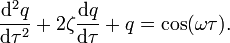
The equation

is known as the universal oscillator equation since all second order linear oscillatory systems can be reduced to this form. This is done through nondimensionalization.
If the forcing function is f(t) = cos(ωt) = cos(ωtcτ) = cos(ωτ), where ω = ωtc, the equation becomes
The solution to this differential equation contains two parts, the "transient" and the "steady state".
Transient solution
The solution based on solving the ordinary differential equation is for arbitrary constants c1 and c2
1 \ \mbox{(overdamping)} \\ e^{-\zeta\tau} (c_1+c_2 \tau) = e^{-\tau}(c_1+c_2 \tau) & \zeta = 1 \ \mbox{(critical damping)} \\ e^{-\zeta \tau} \left[ c_1 \cos \left(\sqrt{1-\zeta^2} \tau\right) +c_2 \sin\left(\sqrt{1-\zeta^2} \tau\right) \right] & \zeta < src="http://upload.wikimedia.org/math/f/6/5/f65c05c1aed77ef6082d00a66f0d63dc.png" style="border-top-style: none; border-right-style: none; border-bottom-style: none; border-left-style: none; border-width: initial; border-color: initial; vertical-align: middle; margin-top: 0px; margin-right: 0px; margin-bottom: 0px; margin-left: 0px; ">
The transient solution is independent of the forcing function. If the system is critically damped, the response is independent of the damping.
Equivalent systems
Harmonic oscillators occurring in a number of areas of engineering are equivalent in the sense that their mathematical models are identical (see universal oscillator equation above). Below is a table showing analogous quantities in four harmonic oscillator systems in mechanics and electronics. If analogous parameters on the same line in the table are given numerically equal values, the behavior of the oscillators will be the same.
| Translational Mechanical | Torsional Mechanical | Series RLC Circuit | Parallel RLC Circuit |
|---|---|---|---|
Position  | Angle  | Charge  | Voltage  |
Velocity  | Angular velocity  | Current  |  |
Mass  | Moment of inertia  | Inductance  | Capacitance  |
Spring constant  | Torsion constant  | Elastance  | Susceptance  |
Friction  | Rotational friction  | Resistance  | Conductance  |
Drive force  | Drive torque  | |  |
Undamped resonant frequency  : : | |||
 |  |  | |
| Differential equation: | |||
 |  |  |  |
Applications
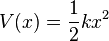
The problem of the simple harmonic oscillator occurs frequently in physics because a mass at equilibrium under the influence of any conservative force, in the limit of small motions, will behave as a simple harmonic oscillator.
A conservative force is one that has a potential energy function. The potential energy function of a harmonic oscillator is:
Given an arbitrary potential energy function V(x), one can do a Taylor expansion in terms of x around an energy minimum (x = x0) to model the behavior of small perturbations from equilibrium.

Because V(x0) is a minimum, the first derivative evaluated at x0 must be zero, so the linear term drops out:

The constant term V(x0) is arbitrary and thus may be dropped, and a coordinate transformation allows the form of the simple harmonic oscillator to be retrieved:
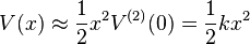
Thus, given an arbitrary potential energy function V(x) with a non-vanishing second derivative, one can use the solution to the simple harmonic oscillator to provide an approximate solution for small perturbations around the equilibrium point.
Further reading
- Serway, Raymond A.; Jewett, John W. (2003). Physics for Scientists and Engineers. Brooks/Cole. ISBN 0-534-40842-7.
- Tipler, Paul (1998). Physics for Scientists and Engineers: Vol. 1 (4th ed. ed.). W. H. Freeman. ISBN 1-57259-492-6.
- Wylie, C. R. (1975). Advanced Engineering Mathematics (4th ed. ed.). McGraw-Hill. ISBN 0-07-072180-7.


Tidak ada komentar:
Posting Komentar