
Most of us have heard of the Socratic method of teaching at one time or another- it's the technique Socrates famously used to educate Athenian youth back in ancient Greece. This method entails the teacher asking the student a series of leading questions sequenced in such a way that the student is able to discover knowledge for him or her self.
I would argue that Physics by Inquiry, a three volume textbook series by Lillian McDermott and the Physics Education Group at the University of Washington, makes spectacularly successful use of a modified form of the Socratic Method.
I would argue that Physics by Inquiry, a three volume textbook series by Lillian McDermott and the Physics Education Group at the University of Washington, makes spectacularly successful use of a modified form of the Socratic Method.
Unlike most textbooks, Physics by Inquiry directly gives the reader very little information. Instead, students using this text book are meant to work in groups with guidance from an instructor to answer leading questions through experiment and reasoning.

Physics Drill for High School Final Exam - Natural Science Program
- Code A
- Download Questions, Download Solutions Code B
- Download Questions, Download Solutions
I first used Physics by Inquiry as a graduate student in a teacher education program, and I found it revelatory. It was exciting and challenging. Equations and calculations were not center stage- ideas were, and those ideas made sense. For the first time in my life, I liked physics. Physics by Inquiry is in fact written largely for pre-and in-service teachers who are furthering their own educations. It seems fairly clear that one point of the books' is to show these current and future teachers just how effective inquiry-based learning can be. It's a lesson that worked for me- I've enthusiastically taken many of the ideas in Physics by Inquiry to heart. The other target audience of these books is college students who lack a strong science background and want to learn introductory physics for any reason.
Although the physics explored in these books is fairly basic, and includes the same topics that you would expect to find in a high school physics course, including properties of matter, heat and temperature, magnets, electric circuits, light and optics, kinematics, and astronomy, the books are not really for high school students. From a purely intellectual perspective, the material would be suitable for a high school class, but it would not be practical in most classrooms because of the high level of independent work it requires from groups. For many, maybe most, high school teachers using the Physics by Inquiry curriculum in unmodified form would be a classroom management disaster. Using the ideas in the book in a modified format however, could be enormously successful.
(Although I wouldn't want to use an unmodified Physics by Inquiry curriculum in most high schools, I would certainly recommend it to a homeschool group, if they have a teacher who is knowledgeable enough to use it.)
Another practical problem with the Physics by Inquiry format is that it is relatively time-consuming. One could make a strong argument that quality of learning matters more that quantity of topics covered, but when students must take standardized exams at the end of the year, that argument begins to feel weak.
As a tutor, I try to be very mindful of the lessons I learned from these books: knowledge really is more powerful when it is created by the student and skillful questioning can lead to excellent results. Physics by Inquiry is a book that I can wholeheartedly recommend to teachers, homeschooling parents, and those curious about physics or the process of scientific inquiry.
Sumber:
http://physics-courses.blogspot.com
Disusun Ulang Oleh:
Arip Nurahman
Pendidikan Fisika, FPMIPA. Universitas Pendidikan Indonesia
&
Follower Open Course Ware at MIT-Harvard University. Cambridge. USA.

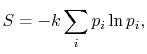

![$\displaystyle = -k \sum_{i=1}^\Omega \frac{1}{\Omega}\ln\left(\frac{1}{\Omega}\... ...ega}\ln\left(\frac{1}{\Omega}\right)\right] =-k\ln\left(\frac{1}{\Omega}\right)$](http://web.mit.edu/16.unified/www/FALL/thermodynamics/notes/img938.png)
![$\displaystyle S=-3k\left[\frac{1}{3}\ln\left(\frac{1}{3}\right)\right]$](http://web.mit.edu/16.unified/www/FALL/thermodynamics/notes/img968.png)

