Rabu, 08 Desember 2010

Termodinamika


7.6 Summary and Conclusions

  1. Entropy as defined from a microscopic point of view is a measure of randomness in a system.
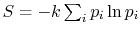
  2. The entropy is related to the probabilities $ p_i$ of the individual quantum states of the system by

    $\displaystyle S =-k\sum_i p_i\ln p_i,$

    where $ k$ 
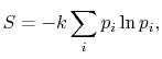
, the Boltzmann constant, is given by $ \mathbf{R}/ N_\textrm{Avogadro}$ .
  3. For a system in which there are $ \Omega$ quantum states, all of which are equally probable (for which the probability is $ p_i =1/\Omega$ ), the entropy is given by

    $\displaystyle S=k\ln\Omega.$

    The more quantum states, the more the randomness and uncertainty that a system is in a particular quantum state.
  4. From the statistical point of view there is a finite, but exceedingly small possibility that a system that is well mixed could suddenly ``unmix'' and that all the air molecules in the room could suddenly come to the front half of the room. The unlikelihood of this is well described by Denbigh [Principles of Chemical Equilibrium, 1981] in a discussion of the behavior of an isolated system:
    ``In the case of systems containing an appreciable number of atoms, it becomes increasingly improbable that we shall ever observe the system in a non-uniform condition. For example, it is calculated that the probability of a relative change of density, $ \Delta \rho/\rho$ , of only $ 0.001\%$ in $ 1\textrm{ cm}^3$ of air is smaller than $ 10^{-10^{8}}$ and would not be observed in trillions of years. Thus, according to the statistical interpretation the discovery of an appreciable and spontaneous decrease in the entropy of an isolated system, if it is separated into two parts, is not impossible, but exceedingly improbable. We repeat, however, that it is an absolute impossibility to know when it will take place.''
  5. The definition of entropy in the form $ S =-k\sum_i p_i\ln p_i$ arises in other aerospace fields, notably that of information theory. In this context, the constant $ k$ is taken as unity and the entropy becomes a dimensionless measure of the uncertainty represented by a particular message. There is no underlying physical connection with thermodynamic entropy, but the underlying uncertainty concepts are the same.
  6. The presentation of entropy in this subject is focused on the connection to macroscopic variables and behavior. These involve the definition of entropy given in Chapter 5 of the notes and the physical link with lost work, neither of which makes any mention of molecular (microscopic) behavior. The approach in other sections of the notes is only connected to these macroscopic processes and does not rely at all upon the microscopic viewpoint. Exposure to the statistical definition of entropy, however, is helpful as another way not only to answer the question of ``What is entropy?'' but also to see the depth of this fundamental concept and the connection with other areas of technology.


Disusun Ulang Oleh;

Arip Nurahman

Pendidikan Fisika, FPMIPA. Universitas Pendidikan Indonesia
&
Follower Open Course Ware at MIT-Harvard University, Cambridge. USA.

Semoga Bermanfaat dan Terima Kasih


Materi kuliah termodinamika ini disusun dari hasil perkuliahan di departemen fisika FPMIPA Universitas Pendidikan Indonesia dengan Dosen:

1. Bpk. Drs. Saeful Karim, M.Si.

2. Bpk. Insan Arif Hidayat, S.Pd., M.Si.

Dan dengan sumber bahan bacaan lebih lanjut dari :

Massachusetts Institute of Technology, Thermodynamics

Professor Z. S. Spakovszk, Ph.D.

Office: 31-265

Phone: 617-253-2196

Email: zolti@mit.edu

Aero-Astro Web: http://mit.edu/aeroastro/people/spakovszky

Gas Turbine Laboratory: home

Ucapan Terima Kasih:

Kepada Para Dosen di MIT dan Dosen Fisika FPMIPA Universitas Pendidikan Indonesia

Semoga Bermanfaat

Selasa, 07 Desember 2010

Termodinamika

Reynolds and Perkins give a numerical example which illustrates the above concepts and also the tendency of a closed isolated system to tend to equilibrium. The starting point is a system in an initial microscopic state that is not an equilibrium distribution. We expect the system will change quantum state, with disorder, randomness growing until they reach the equilibrium values. The specific system to be studied is composed of 10 particles $ A$ , $ B$ , $ C$ , ..., $ J$ , each of which can exist in one of 5 states, of energies 0, 1, 2, 3, 4. The system is isolated and has a total energy of 30. The total energy remains unchanged during the evolution of the microscopic states. Some of the allowed states are shown in Figure 7.1

Figure 7.1: Some allowed states of the system in the numerical example. Note each state has a total energy of 30. [Reynolds and Perkins, 1977]
Image fig4EntropyStates_web
Figure 7.2: Constant energy state groups [Reynolds and Perkins, 1977]
Image fig4ConstantEnergyStateGroups_web

For ten particles, 4 energy states, and a total energy of 30, there are 72,403 possible quantum states (4 states are indicated in Figure 7.1). However, there are only 23 possible distributions in terms of the number of particles having a given energy as shown in Figure 7.2. For example, states 2 and 3 in Figure 7.1 are two different quantum states, but they represent the same group (22) in Figure 7.2. The allowed state groups

If the quantum-state probabilities are equal, each quantum state has a probability of 1/72,403. The probabilities of each group are thus directly proportional to the number of quantum states in this group. For instance, group 22 has 90 quantum states, so its probability is $ 90/72,403 \cong 0.0012$ . We now know what the equilibrium distribution of probabilities is. We now address the time evolution of a system to the equilibrium state. To see this, we start a system from one of the 22 non-equilibrium groups and track the behavior over time. A way to examine the process is to consider what happens if two particles interact, doing this numerically for the instantaneous quantum state. The two particles are free to change energy as long as the total energy of the system is conserved. This may or may not end up by changing the state group (the particles could interact and only switch states). There are 45 possible pairs for this interaction (there are $ 10 \times 9$ possible ways to carry out the interaction, but two of them, say interactions between $ A$ and $ D$ and $ D$ and $ A$ , are the same), and we assume that any of them is equally likely to happen.

If the system is initially in state 1 of Figure 7.1, it is in group 23 of Figure 7.2. For each of the 45 pairs, there are two interactions that take the system to group 22, and one that leaves the system unchanged. (For interactions between $ A$ and $ D$ , say, the result can be that $ A$ and $ D$ have their energy unchanged, that $ A$ loses energy and $ D$ gains energy, or that $ A$gains energy and $ D$ loses energy. In the first of these, the system will remain in group 23. In the second and third it will move to group 22.) Hence the transition probability from group 23 to group 22 is $ 2/3$ , and the transition probability from 23 to 23 is $ 1/3$ .

Figure 7.3: Transition probabilities (probability for transition from initial group to final group) in numerical experiment with isolated system [Reynolds and Perkins, 1977]
Image fig4TransitionProbabilities_web

For the other groups, the transitions are more complicated, but can be found numerically, with the results shown in Figure 7.3. The numerical experiments were carried out with the system initially in state 23 and with successive interactions chosen randomly in accordance with the transition probabilities of Figure 7.3. The experiment was repeated 10,000 times, with a different group history traced out each time and, again, the system energy maintained at 30. The fraction of the experiments in which each group occurred at time $ t$ was used to calculate the group probabilities $ p_k(t)$ at each time. The entropy was then found for the distribution $ p_k$ at that time.

Figure 7.4: Evolution of the probability distribution with time (interaction number) [Reynolds and Perkins, 1977]
Image fig4ProbabilityEvolutionOverTime_web

Figure 7.4 shows the evolution of some of the $ p_k(t)$ with time (the unit of time is the interaction number for the calculations) starting from group 23. After roughly ten interactions, the probabilities have reached a steady-state level, which are the equilibrium probabilities from Figure 7.2.

Figure 7.5: Entropy for the system as a function of time [Reynolds and Perkins, 1977]
Image fig4EntropyOverTime_web

The computed entropy is given in Figure 7.5 as a function of time. It increases to the equilibrium value with the same sort of behavior as the probability distribution.

The interactions allow the system to change groups. The transition probabilities are large for groups with high equilibrium probabilities.

There is one additional aspect of the behavior that is brought out in the text. This is the difference in overall probabilities between the order of transitions. The probability of a transition sequence is the product of the individual step transition probabilities. The transition 23-22-12-9-1 thus has the probability: $ 0.667 \times 0.4148 \times 0.2222 \times 0.1333 = 8.191 \times 10^{-3}$ . The reverse transition, 1-9-12-22-23 has the probability: $ 0.0444 \times 0.0667 \times 0.0296 \times 0.0074 = 6.5 \times 10^{-7}$ . There is an enormous probability that the system will move towards (and persist in) quantum state groups that have high equilibrium probabilities. Once a system has moved out of group 23, there is little likelihood that it will ever return. Further, for engineering systems, which have not 10 particles, but upwards of $ 10^{20}$ , the difference between transitions and their reverses are much more marked, and the probability is overwhelming that the distribution will be a quantum state with a broad distribution of particle energies.


Disusun Ulang Oleh:

Arip Nurahman

Pendidikan Fisika, FPMIPA. Universitas Pendidikan Indonesia

&

Follower Open Course Ware at MIT-Harvard University. Cambridge. USA.


Materi kuliah termodinamika ini disusun dari hasil perkuliahan di departemen fisika FPMIPA Universitas Pendidikan Indonesia dengan Dosen:

1. Bpk. Drs. Saeful Karim, M.Si.

2. Bpk. Insan Arif Hidayat, S.Pd., M.Si.

Dan dengan sumber bahan bacaan lebih lanjut dari :

Massachusetts Institute of Technology, Thermodynamics

Professor Z. S. Spakovszk, Ph.D.

Office: 31-265

Phone: 617-253-2196

Email: zolti@mit.edu

Aero-Astro Web: http://mit.edu/aeroastro/people/spakovszky

Gas Turbine Laboratory: home

Ucapan Terima Kasih:

Kepada Para Dosen di MIT dan Dosen Fisika FPMIPA Universitas Pendidikan Indonesia

Semoga Bermanfaat

Senin, 06 Desember 2010

Termodinamika


7.4 Connection between the Statistical Definition of Entropy and Randomness

We need now to examine the behavior of the statistical definition of entropy as regards randomness. Because a uniform probability distribution reflects the largest randomness, a system with $ n$ allowed states will have the greatest entropy when each state is equally likely. In this situation, the probabilities become

$\displaystyle p_i = p = \frac{1}{\Omega},$(7..15)

where $ \Omega$ is the total number of microstates. The entropy is thus
$\displaystyle S$$\displaystyle = -k \sum_{i=1}^\Omega \frac{1}{\Omega}\ln\left(\frac{1}{\Omega}\... ...ega}\ln\left(\frac{1}{\Omega}\right)\right] =-k\ln\left(\frac{1}{\Omega}\right)$

$\displaystyle = k \ln\Omega.$(7..16)

Equation (7.16) states that the larger the number of possible states the larger the entropy. The behavior of the entropy stated in Equation (7.16) can be summarized as follows:
  1. $ S$ is maximum when $ \Omega$ is maximum, which means many permitted quantum states, hence much randomness,
  2. $ S$ is minimum when $ \Omega$ is minimum. In particular, for $ \Omega=1$ , there is no randomness and $ S=0$ .
These trends are in accord with our qualitative ideas concerning randomness. Equation (7.16) is carved on Boltzmann's tombstone (he died in 1906 in Vienna).

We can also examine the additive property of entropy with respect to probabilities. If we have two systems, $ A$ and $ B$ , which are viewed as a combined system, $ C$ , the quantum states for the combined system are the combinations of the quantum states from $ A$ and $ B$ . The quantum state where $ A$ is in its state $ x$ and $ B$ is in its state $ y$ would have a probability $ p_{Ax}\cdot p_{By}$ because the two probabilities are independent. The number of probabilities for the combined system, $ \Omega_C$ , is thus defined by $ \Omega_C=\Omega_A\cdot \Omega_B$ . The entropy of the combined system is

$\displaystyle S_C =k\ln(\Omega_A\Omega_B)=k\ln\Omega_A+k\ln\Omega_B =S_A+S_B$(7..17)

Equation (7.16) is sometimes taken as the basic definition of entropy, but it should be remembered that it is only appropriate when each quantum state is equally likely. Equation (7.12) is more general and applies equally for equilibrium and non-equilibrium situations.

A simple numerical example shows trends in entropy changes and randomness for a system which can exist in three states. Consider the five probability distributions

$\displaystyle (i)\:p_1$$\displaystyle =1.0,$$\displaystyle p_2$$\displaystyle =0,$$\displaystyle p_3$$\displaystyle =0;$$\displaystyle S=-k(1\ln(1)+0\ln(0)+0\ln(0))$$\displaystyle =0$
$\displaystyle (ii)\:p_1$$\displaystyle =0.8,$$\displaystyle p_2$$\displaystyle =0.2,$$\displaystyle p_3$$\displaystyle =0;$$\displaystyle S=-k(0.8\ln(0.8)+0.2\ln(0.2)+0\ln(0))$$\displaystyle =0.5k$
$\displaystyle (iii)\:p_1$$\displaystyle =0.8,$$\displaystyle p_2$$\displaystyle =0.1,$$\displaystyle p_3$$\displaystyle =0.1;$$\displaystyle S=-k(0.8\ln(0.8)+0.1\ln(0.1)+0.1\ln(0.1))$$\displaystyle =0.6k$
$\displaystyle (iv)\:p_1$$\displaystyle =0.5,$$\displaystyle p_2$$\displaystyle =0.3,$$\displaystyle p_3$$\displaystyle =0.2;$$\displaystyle S=-k(0.5\ln(0.5)+0.3\ln(0.3)+0.2\ln(0.2))$$\displaystyle =1.0k$
$\displaystyle (v)\:p_1$$\displaystyle =1/3,$$\displaystyle p_2$$\displaystyle =1/3,$$\displaystyle p_3$$\displaystyle =1/3;$$\displaystyle S=-3k\left[\frac{1}{3}\ln\left(\frac{1}{3}\right)\right]$$\displaystyle =1.1k$

The first distribution has no randomness. For the second, we know that state 3 is never found. Distributions (iii) and (iv) have progressively greater uncertainty about the distribution of states and thus higher randomness. Distribution (v) has the greatest randomness and uncertainty and also the largest entropy.

Disusun Ulang Oleh:

Arip Nurahman

Pendidikan Fisika, FPMIPA. Universitas Pendidikan Indonesia

&

Follower Open Course Ware at MIT-Harvard University. Cambridge. USA.


Materi kuliah termodinamika ini disusun dari hasil perkuliahan di departemen fisika FPMIPA Universitas Pendidikan Indonesia dengan Dosen:

1. Bpk. Drs. Saeful Karim, M.Si.

2. Bpk. Insan Arif Hidayat, S.Pd., M.Si.

Dan dengan sumber bahan bacaan lebih lanjut dari :

Massachusetts Institute of Technology, Thermodynamics

Professor Z. S. Spakovszk, Ph.D.

Office: 31-265

Phone: 617-253-2196

Email: zolti@mit.edu

Aero-Astro Web: http://mit.edu/aeroastro/people/spakovszky

Gas Turbine Laboratory: home

Ucapan Terima Kasih:

Kepada Para Dosen di MIT dan Dosen Fisika FPMIPA Universitas Pendidikan Indonesia

Semoga Bermanfaat